Week 3 - Solving second order ODEs

*SOLVING SECOND ORDER DIFFERINCAL EQUATION

clear all 
close all
clc


b=0.05;
g=9.81;
l=1;
m=1;

%initial condition
theta_0=[0;3];

%time points
t_span=linspace(0,20,500);

 % solve ode
[t,results]= ode45(@(t,theta) ode_func(t,theta,b,g,l,m),t_span,theta_0);

% plotting
figure(1)
hold on
plot(t,results(:,1))
plot(t,results(:,2))

ylabel('plot')
xlabel('time(seconds)')


ct=1;

for i=1:length(results(:,1))
    X_start=0
    Y_start=0
    X_end=l*sin(results(i,1))
    Y_end=-l*cos(results(i,1))


figure(2)
plot([-1 1],[0 0],'linewidth',5)
hold on;
plot([X_start X_end], [Y_start Y_end],'LineWidth',3)
hold on;
plot(X_end,Y_end,'o','MarkerSize',20,'MarkerFaceColor','y')
title('animation of pendulam')
axis([-1.5 1.5 -1.5 1])
pause(0.0003)
hold off;
end

M(ct)= getframe(gcf);
ct=ct+1;


movie(M)
videofile=VideoWriter('pendulam animation.avi','Uncompressed AVI')
open(videofile)
writeVideo(videofile,M)
close(videofile)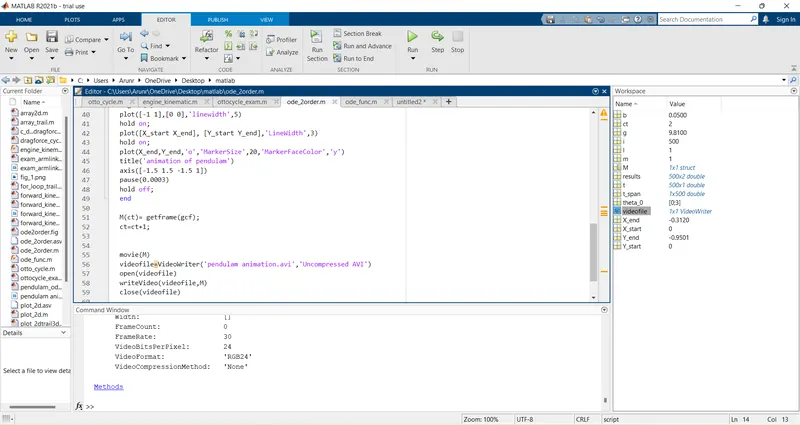

VIDEO LINK

https://drive.google.com/file/d/1q3l7T-SAUXGX8kl0rBOY45A5NJdbly6P/view?usp=sharing

EXPLANATION

As we know the fixed parameter length , mass, damping coefficient ,accleration,gravity.

time is taken between 0 to 20 sec

by using ode45 command ODE function is introduced

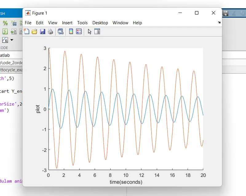
by ploting we can see displacement in y axis against time in x axis

we can reduced the displacement by reducing damp coefficient

by using the loop command mass at various points and at various time are marked in the graph and are ploted

by using movie command we can save it to avi.file.....