Week 6: Conjugate Heat Transfer Simulation
Introduction:
CONJUGATE HEAT TRANSFER:
The term conjugate heat transfer (CHT) is used to describe processes which involves variation of temperature within solid and fluids due to thermal interaction between the solid and fluid. the exchange of thermal energy between the two physical bodies is called study of heat transfer the rate of transferred heat is directly proportional to the temp difference between the bodies. Conjugate heat transfer corresponds with combination of heat transfer in solids and heat transfer in fluids. In solids conduction often dominates whereas in fluids ,convection usually dominates. Efficiency combining heat transfer in fluids and solids is the key to designing effective coolers, heaters, or heat exchangers.
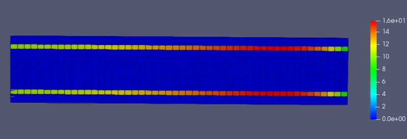
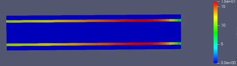
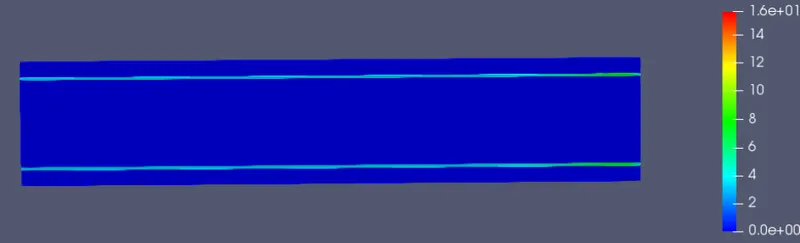
Importance of Y+:
The y+ values denotes where in the y+ vs u+ curve we are respect to the cell size. it is undesirable to have cell size that leads to a y+ of between 10 to 30 since the modelling of flow transitioning from laminar to turbulent is not easy and is still being researched. due to this fact it is better to have y+ of less than 10 meaning we be at the laminar region or have a y+ of greater than 30 where we can go with a wall function and still achives results. The y+ value can be used as marked based on which we can decide on the base grid size and make a decision based on the computing power as to whether the grid needs to be refined further or coarsened.
GEOMETRY:
Geometry is crated in converge studio with center1(0,0,0) and center2(0,0,0.2) with inner radius of 0.015 and outer radius of 0.02m.
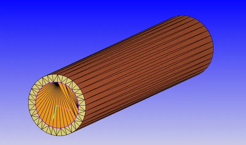
geometry with different region:
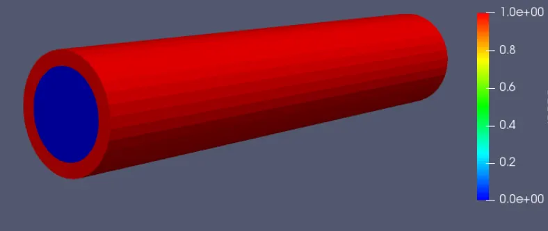
CASE SETUP:
Material: predefined mixture :air
species: gas=o2,n2
solid =aluminium
Run parameters: solver= transient
Simulation time parameter: Start time=0s
End time=0.5s
Initial time step=1e-7s
Minimum time step=1e-7s
Maximum time step=1s
Initial velocity calculation:
Rn=7000.
At 25 deg C, properties of air are: Density=1.184 kg/m^3
Dynamic viscosity=1.86e-5 pa.s
Radius of cyclinder=0.015m
Re=(rho*V*D)/Dynamic viscosity
7000=(1.184*V*0.03)/(1.86e-5)
V=3.665 m/s
Region & initialization:
Stream id=0 is Fluid region
Velocity=3.665 m/s(z-direction)
temperature=300k
pressure=1.1325 pa
species=air(O2,N2)
stream in=1 is solid region
temperature=300k
BOUNDARY CONDITION:
1 Solid outer wall: type=wall
velocity :slip
temp=heat flux
flux=-10000(negative shows heat is going inside the system)
2 thickness solid region:type wall
velocity:slip
temp=zero noraml gradient
3 inlet fluid region: type=inflow
velocity=3.665m/s(z-direction)
pre3ssure=zero normal gradient
spicies=Air(O2,N2)
4Outlet fluid region:type= outflow
pressure=101325 pa
temp=300k
species=air(O2,N2)
5 Intreface:it is a boundary type which sepearte two rype of material or phase.
Forward region:region: fluid region
velocity:law of wall
temp=law of wall
Reverse region:region:solid region
velocity=law of wall
temp=specified value
turbulence model :RNG K-e
Super cycling modelling:
Super cycling is method used by converge to deal with conjugate heat transfer problem. time required for fluid solver to reach steday state is much smaller than that taken by solid hence it will create the pronlem for solid side solver as it will not reach steday state in provided time. Hence we need to pause fluid solver until solid solver reach steady state.
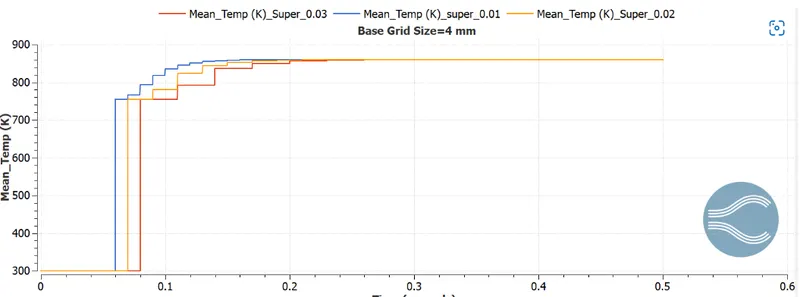
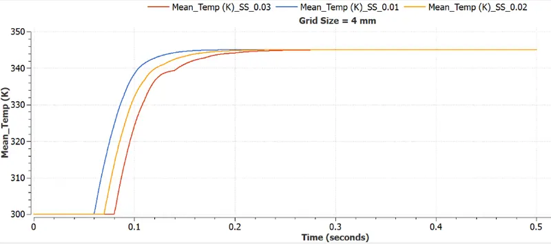
To understand super cycling effect set supercycle stage interval to 0.01,0.02,0.03
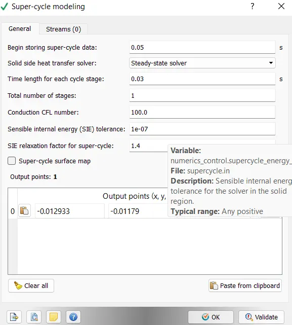
BASE GRID:
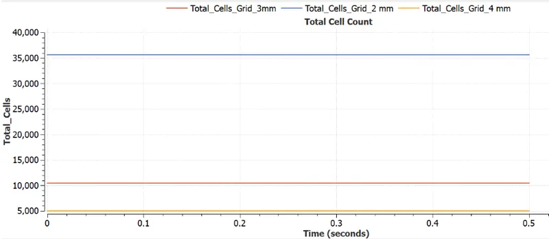
OF 0.004m, 0.003m, 0.002m
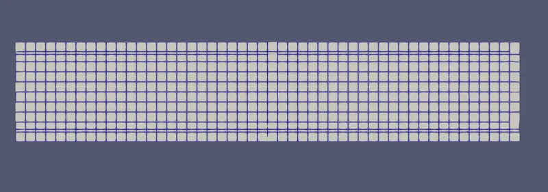
0.003m
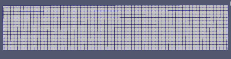
0.002m
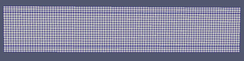
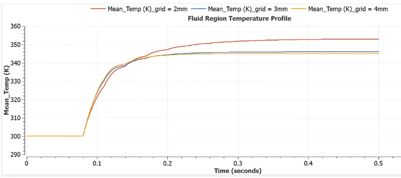
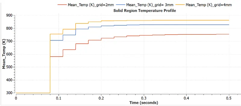
Temperature plots for fluid and solid region:
following temp plots are taken at super cycle stage of 0.03.
CELL COUNT:
Y+:
Grid size=0.004m
0.003m
0.002m
SUPERCYCLE STAGE INTERVAL:
Super cycling is method used by converge to deal with conjugate heat transfer problem. time required for fluid solver to reach steady state is much smaller than that taken by solid solver hence it will createproblem for solid side solver as it will not reach steady state in provided time. hence we need to pause fluid solver untill solid solver reach steady state. Here transient solver solve both fluid and solid region for initial steps and stores the heat transfer coefficient and temp at interface boundary condition and run steady state solver for solid region untill it reaches steady state.
for solid region:
for fluid region:
ANIMATION:
ITS IS OF 0.004m GRID SIZE:
temperature animation:
pressure animation:
velocity animation: