Week 7 - Simulation of a 1D Super-sonic nozzle flow simulation using Macormack Method
SIMULATION OF 1D SUPERSONIC FLOW NOZZLE USING MACROMAC METHOD:
*NON CONSERVATION FORM OF GOVERNING EQUATION:
CONTINUITY EQUATION

MOMENTUM EQUATION

ENERGY EQUATION

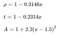
All the variables are non dimensional form.
initial condition
CONSERVATION FORM OF GOVERNING EQUATION
COUNTIUNITY EQUATION
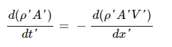
MOMENTUM EQUATION

ENERGY EQUATION

The above equation can be simplfy into the following equation
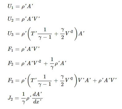
where u1,u2,u3 are called the dolution vector, and F1,F2,F3 are the flux vector and j2 is called the source term.
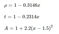
INITIAL CONDITION
MATLAB CODE
clear all

close all
clc
n=31;
x=linspace(0,3,n);
tol=1e-4;
m_analytical=0.579*ones(1,n);
[m_nc]=supersonic_non_conservative(n,tol);
[m_c]=supersonic_conservative(n,tol);
figure(5)
plot(x,m_nc,'linewidth',2)
hold on
plot(x,m_c,'linewidth',2)
hold on
plot(x,m_analytical,'linewidth',2)
title('mass flow rate vs x')
xlabel('x')
ylabel('mass flow rate')
legend('non conservative','conservative','analytical')
function for non conservative
function [m_mc]=supersonic_non_conservative(n,tol)
tic
%grid
x=linspace(0,3,n);

dx=x(2)-x(1);
gamma=1.4;
%specific throat
throat =(n+1)/2;
m_analytical=0.579*ones(1,n);

c=0.5;
%initial profiles
rho=1-0.3146*x;
t=1-0.2314*x;  % temperature
v=(0.1+1.09*x).*t.^0.5;
rho_old=rho'
v_old=v;
t_old=t;
%area
a=1+2.2*(x-1.5).^2;
%time steps
nt=1400;
nt_step=linspace(1,nt,nt);
for p=1:n
    dt_a(p)=c*dx/(t(p)^0.5+v(p));
end
dt=min(dt_a);
%outer time loop
iter=1;
error_rho=9e9;
error_v=9e9;
error_t=9e9;
for k=1:nt
    rho_old=rho;
    v_old=v;
    t_old=t;

    %predictor method
    for j=2:n-1
        dvdx=(v(j+1)-v(j))/dx;
        drhodx=(rho(j+1)-rho(j))/dx;
        dtdx=(t(j+1)-t(j))/dx;
        dlogadx=(log(a(j+1))-log(a(j)))/dx;

        % countinuity equation
        drhodt_p(j)=-rho(j)*dvdx-rho(j)*v(j)*dlogadx-v(j)*drhodx;

        %momentumequation
        dvdt_p(j)=-v(j)*dvdx-(1/gamma)*(dtdx+(t(j)/rho(j))*drhodx);

        %energy equation
        dtdt_p(j)=-v(j)*dtdx-(gamma-1)*t(j)*(dvdx+v(j)*dlogadx);

        % solution update
        rho(j)=rho(j)+drhodt_p(j)*dt;
        v(j)=v(j)+dvdt_p(j)*dt;
        t(j)=t(j)+dtdt_p(j)*dt;
    end
    %corrector method
     for j=2:n-1
        dvdx=(v(j)-v(j-1))/dx;
        drhodx=(rho(j)-rho(j-1))/dx;
        dtdx=(t(j)-t(j-1))/dx;
        dlogadx=(log(a(j))-log(a(j-1)))/dx;

        % countinuity equation
        drhodt_c(j)=-rho(j)*dvdx-rho(j)*v(j)*dlogadx-v(j)*drhodx;

        %momentumequation
        dvdt_c(j)=-v(j)*dvdx-(1/gamma)*(dtdx+(t(j)/rho(j))*drhodx);

        %energy equation
        dtdt_c(j)=-v(j)*dtdx-(gamma-1)*t(j)*(dvdx+v(j)*dlogadx);
     end

     % compute avg time deravative
     drhodt=0.5*(drhodt_p+drhodt_c);
     dvdt=0.5*(dvdt_p+dvdt_c);
     dtdt=0.5*(dtdt_p+dtdt_c);

     %final solution update
     for i=2:n-1
         rho(i)=rho_old(i)+drhodt(i)*dt;
         v(i)=v_old(i)+dvdt(i)*dt;
         t(i)=t_old(i)+dtdt(i)*dt;
     end
     m=v./t.^0.5;
     m_nc=rho.*a.*v;
     m_nct(k,:)=rho.*a.*v;
     error_rho=max(abs(rho-rho_old));
     error_v=max(abs(v-v_old));
     error_t=max(abs(t-t_old));

     if (error_rho>tol && error_v>tol && error_t>tol)
         iter=iter+1;
     end

     %apply boundary conditions
     %inlet
     v(1)=2*v(2)-v(3);
     rho(n)=2*rho(n-1)-rho(n-2);
     t(n)=2*t(n-1)-t(n-2);

end
rho_throat=rho(throat);
v_throat=v(throat);
m_throat=m(throat);
figure(1)
subplot(4,1,2)
plot(x,rho,'linewidth',2)

xlabel('nozzle length')
ylabel('density ratio')
subplot(4,1,3)
plot(x,v,'r','LineWidth',2)

xlabel('nozzle length')
ylabel('velocity ratio')
subplot(4,1,4)
plot(x,t,'g','LineWidth',2)

xlabel('nozzle length')
ylabel('temperature ratio')
subplot(4,1,1)
plot(x,m,'m','LineWidth',2)
title(sprintf('no of timestep=%d','no of iteration to steady=%d',k,iter))
xlabel('nozzle length')
ylabel('mach number')
subtitle('nonconservative form')

figure(3)
plot(x,m_nct(50,:),x,m_nct(100,:),x,m_nct(200,:),x,m_nct(300,:),x,m_nct(500,:),'o',x,m_analytical,'LineWidth',2)
xlabel('non dimensionless distance x')
ylabel('non dimensionless mass flow rate')
title('variation of mass flow rate (non conservative)')
legend('50dt','100dt','200dt','300dt','700dt','analytical')
time_nc=toc;
fprintf('time of simulation for nonconservative=%gsn',time_nc);
end
function for conservative
function [m_c]=supersonic_conservative(n,tol)
tic
%grid
x=linspace(0,3,n);
dx=x(2)-x(1);
gamma=1.4;
throat=(n+1)/2;
m_analytical=0.579*ones(1,n);
%initial profiles
for q=1:n
    if((x(q)>0) && (x(q)<0.5))
        rho(q)=1;
        t(q)=1;
    elseif ((x(q)<1.5) && (x(q)>0.5))
        rho(q)=1-0.366*(x(q)-0.5);
        t(q)=1-0.167*(x(q)-0.5);
    elseif ((x(q)>=1.5)&& (x(q)<=3.5))
        rho(q)=0.634-0.3879*(x(q)-1.5);
        t(q)=0.833-0.03507*(x(q)-1.5);
    end
end
%area
a=1+2.2*(x-1.5).^2;
v=0.59./(rho.*a);
u1=rho.*a;
u2=rho.*a.*v;
u3=rho.*(t./(gamma-1)+(gamma/2)*v.^2).*a;
%time step
nt=1400;
nt_dtep=linspace(1,nt,nt);
c=0.5;
for p=1:n
    dt_a(p)=c*dx/(t(p)^0.5+v(p));
end
dt=min(dt_a);
%outer time loop
iter=1;
error_rho=9e9;
error_v=9e9;
error_t=9e9;

for k=1:nt
    u1_old=u1
    u2_old=u2;
    u3_old=u3;
    rho_old=u1_old./a;
    v_old=u2_old./u1_old;
    t_old=(gamma-1)*((u3_old./u1_old)-(gamma/2)*v_old.^2);
    f1=u2;
    f2=(u2.^2)./u1+((gamma-1)/gamma)*(u3-(gamma/2)*(u2.^2)./u1);
    f3=(gamma*u2.*u3)./u1-((gamma*(gamma-1)/2)*(u2.^3)./u1.^2);

    %predictor method
    for j=2:n-1
        j2(j)=(1/gamma)*rho(j)*t(j)*(a(j+1)-a(j))/dx;

        %continuity equation
        du1dt_p(j)=-(f1(j+1)-f1(j))/dx;

        %momentumequation
        du2dt_p(j)=j2(j)-(f2(j+1)-f2(j))/dx;

        %energy equation
        du3dt_p(j)=-(f3(j+1)-f3(j))/dx;

        %solution update
        u1(j)=u1(j)+du1dt_p(j)*dt;
        u2(j)=u2(j)+du2dt_p(j)*dt;
        u3(j)=u3(j)+du3dt_p(j)*dt;
    end
    rho=u1./a;
    v=u2./u1;
    t=(gamma-1)*((u3./u1)-(gamma/2)*v.^2);
    f1=u2
    f2=(u2.^2)./u1+((gamma-1)/gamma)*(u3-(gamma/2)*(u2.^2)./u1);
    f3=(gamma*u2.*u3)./u1-((gamma*(gamma-1)/2)*((u2.^3)./(u1.^2)));

    %corrector method
    for j=2:n-1
        j2(j)=(1/gamma)*rho(j)*t(j)*(a(j)-a(j-1))/dx;
        %continuty equation
        du1dt_c(j)=-(f1(j)-f1(j-1))/dx;

        %momentum equation
        du2dt_c(j)=j2(j)-(f2(j)-f2(j-1))/dx;

        %energy equation
        du3dt_c(j)=-(f3(j)-f3(j-1))/dx;

    end

    %compute avg time deravative
    du1dt=0.5*(du1dt_p+du1dt_c);
    du2dt=0.5*(du2dt_p+du2dt_c);
    du2dt=0.5*(du2dt_p+du2dt_c);

    %final solution update
    for i=2:n-1
        u1(i)=u1_old(i)+du1dt(i)*dt;
        u2(i)=u2_old(i)+du2dt(i*dt);
        u3(i)=u3_old(i)+du3dt(i*dt);
    end
    %apply boundary condition
    %inlet
    u1(1)=rho(1).*a(1);
    u2(1)=2*u2(2)-u2(3);
    v(1)=u2(1)/(rho(1)*a(1));
    u3(1)=u1(1)*(t(1)/(gamma-1)+(gamma/2)*v(1)^2);
    %outlet
    u2(n)=2*u2(n-1)-u2(n-2);
    u1(n)=2*u1(n-1)-u1(n-2);
    u3(n)=2*u3(n-1)-u3(n-2);

    %updating values
    rho=u1./a;
    v=u2./u1;
    t=(gamma-1)*((u3./u1)-(gamma/2)*v.^2);
    m=v./t.^0.5;
    m_c=rho.*a.*v;
    m_nc(k,:)=rho.*a.*v;

    error_rho=max(abs(rho-rho_old));
    error_v=max(bas(v-v_old));
    error_t=max(abs(t-t_old));

    if (error_rho>tol && error_v>tol && error_t>tol)
        iter=iter+1;
    end
end
rho_throat=rho(throat);
v_throat=v(throat);
m_throat=m(throat);

figure(2)
subplot(4,1,2)
plot(x,rho,'linewidth',2)

xlabel('nozzle length')
ylabel('density ratio')
subplot(4,1,3)
plot(x,v,'r','LineWidth',2)

xlabel('nozzle length')
ylabel('velocity ratio')
subplot(4,1,4)
plot(x,t,'g','LineWidth',2)

xlabel('nozzle length')
ylabel('temperature ratio')
subplot(4,1,1)
plot(x,m,'m','LineWidth',2)
title(sprintf('no of timestep=%d','no of iteration to steady state=%d',k,iter))
xlabel('nozzle length')
ylabel('mach number')
subtitle('conservative form')

figure(4)
plot(x,m_nc(50,:),x,m_nc(100,:),x,m_nc(200,:),x,m_nc(300,:),x,m_nc(700,:),'o',x,m_analytical,'linewidth',2);
xlabel('non dimensional distance x')
ylabel('non dimensionless mass floe rate')
title('variation of mass flow rate (conservative)')
legend('50dt','100dt','200dt','300dt','700dt','analytical')
time_c=toc;
fprintf('time of simulation for conservative=%gsn',time_c);
end
PLOTS
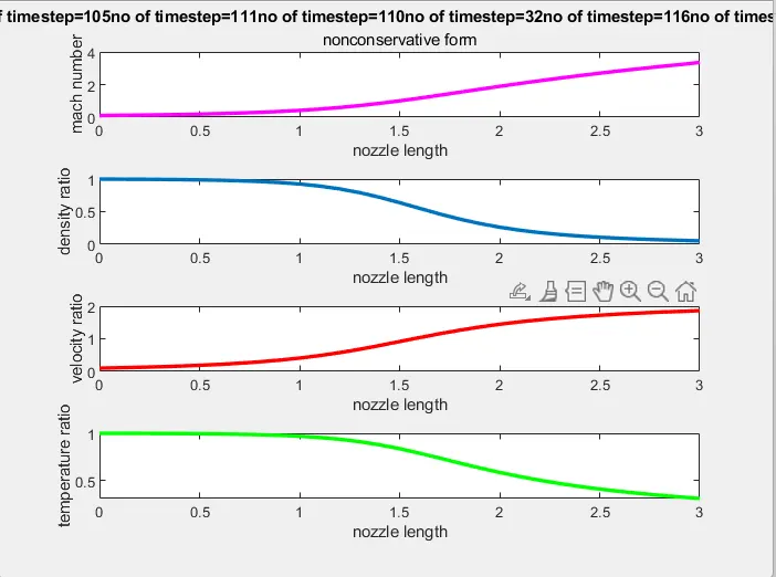
PROFILE FOR FLOW VARIABLE FOR NON CONSERVATIVE FORM
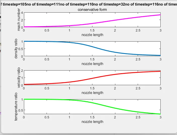
PROFILE FOR FLOW VARIABLE FOR CONSERVATIVE FORM
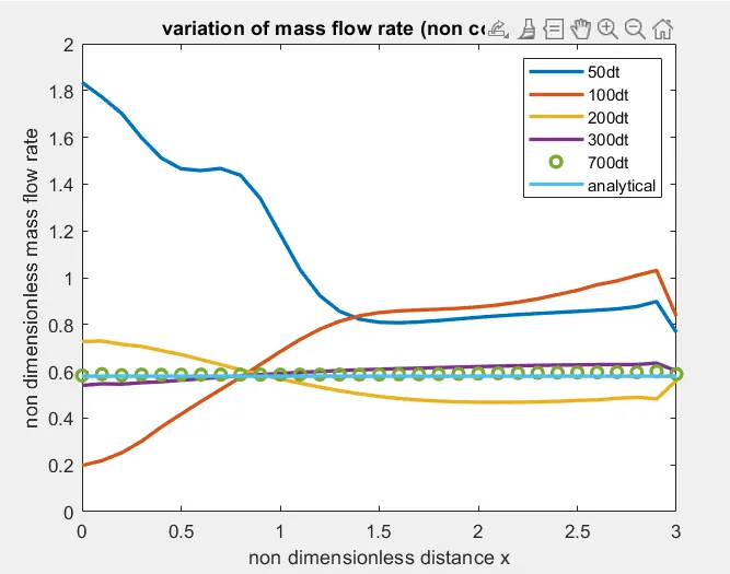
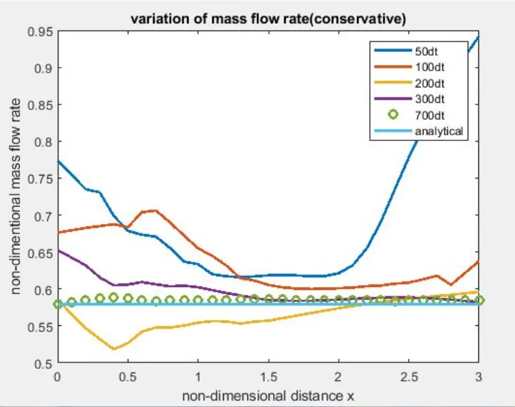
Variable for mass flow rate at different time step
for non conservation
for conservation
convergence:
through the above two graph the converence time step can be analysed we can say that at 700 time step the mass flow rate correspond to the analytical solution that means it reach to steady state solution.
Comparision of mass flow rate between conservative and non conservative
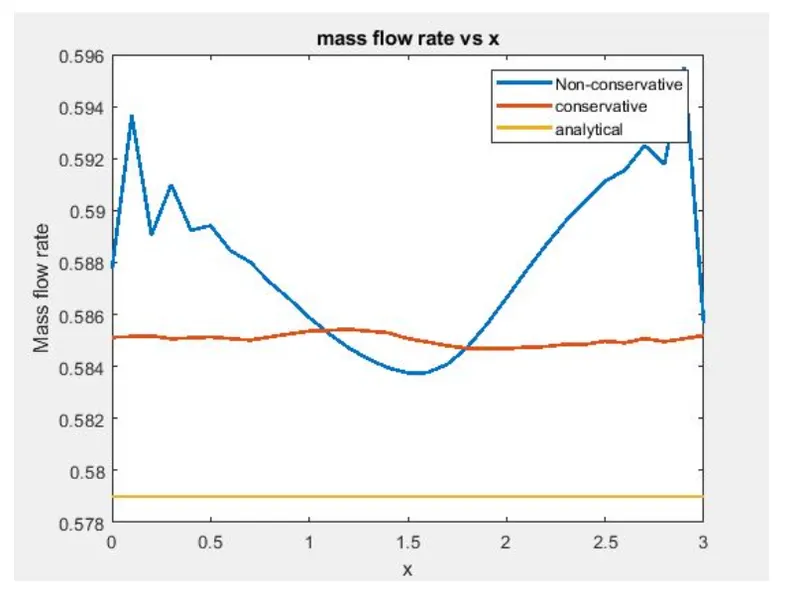
from this we can conclude that mass flow rate in conservative show better result correspond to analytical solution.