Week 4.1: Project - Steady state simulation of flow over a throttle body
PROCEDURE:
step:1
importing the geometry and modifing the geometry suitable for smulation.
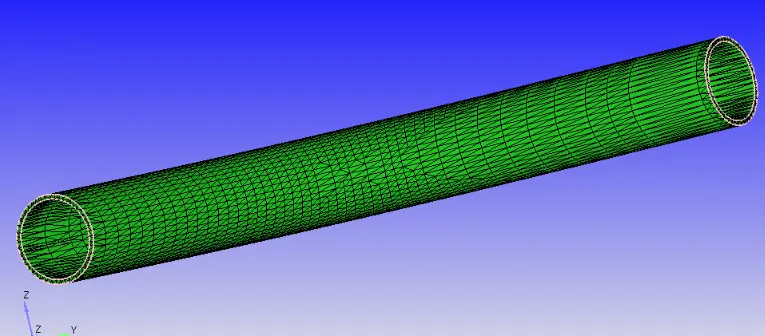
By using the boundary fence option the outer layer is removed so that the free edges are poped and then it is rectified as using patch command.
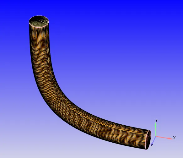
final geometry redy for simulation:
step:2
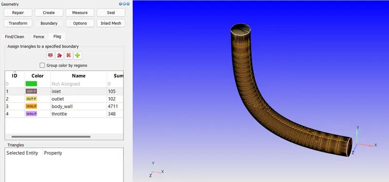
After that give the boundaries once the boundaries have been flagged we assign the different boundary conditions for the flow to take place within the geometry.
step:3
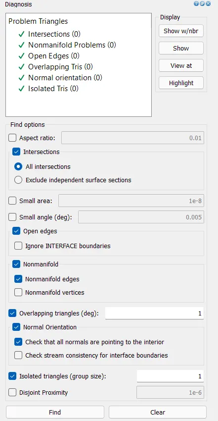
check whether there is any error by using the diagnosis tool.
step 4:
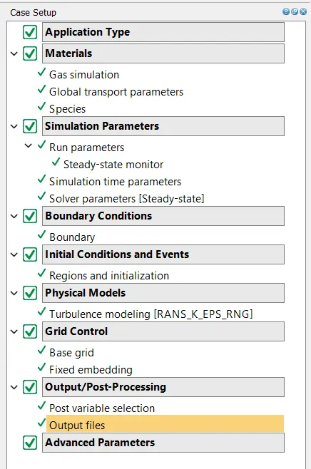
Steps for setting up simulation:
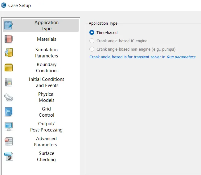
select application time based .
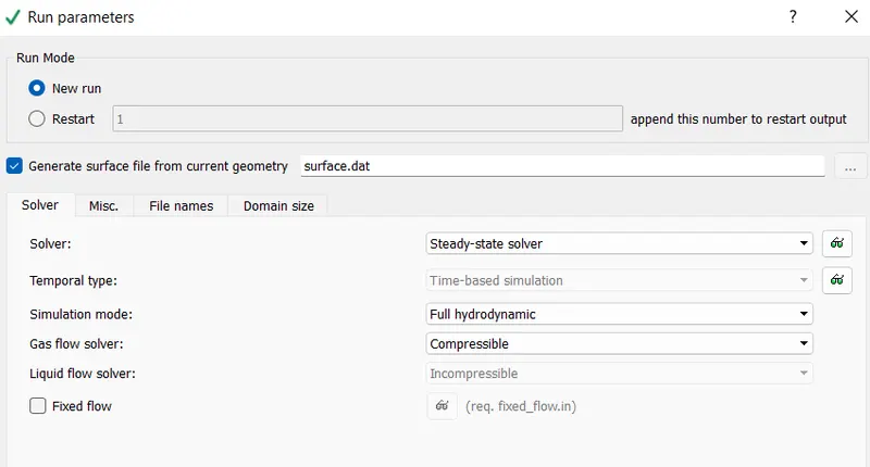
select stedy state solver for simulation and also pressure based.
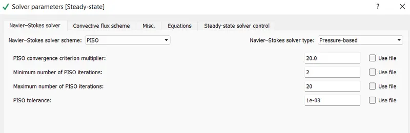
in steady state solver we can give minimum number of cycle for simulation:
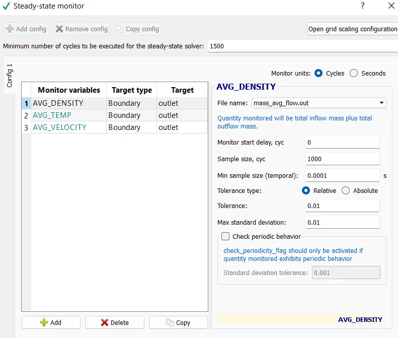
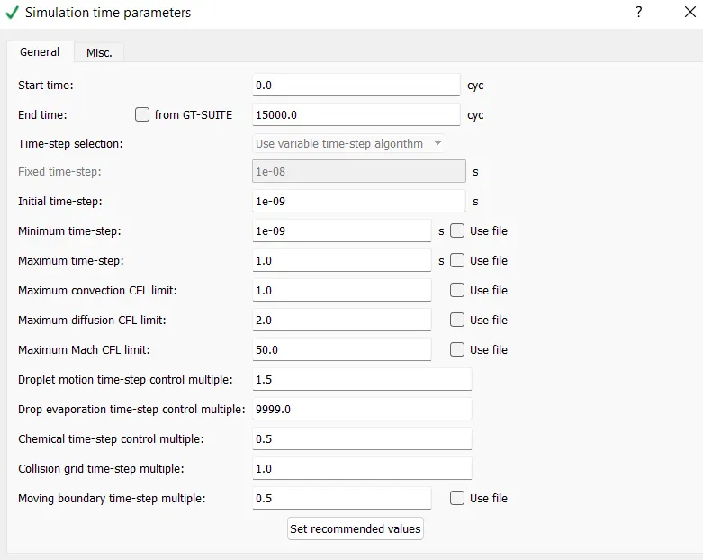
define start and end time for simulation:
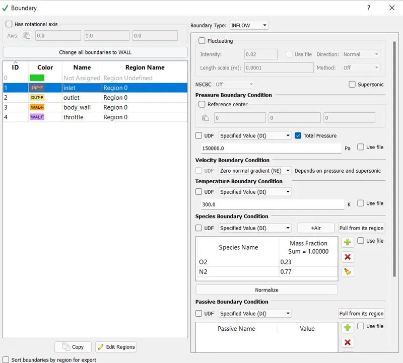
Then after boundary condition are assinged to the region and also the inlet condition are given.
inlet:
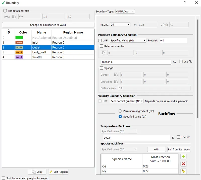
outlet:
throttle:
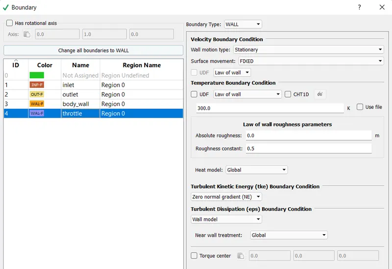
in here wall are defined to law of wall and temperature value is defined.
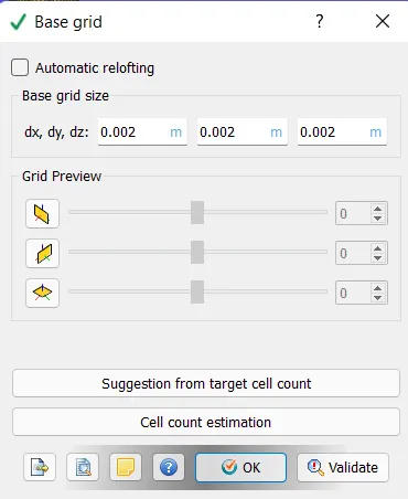
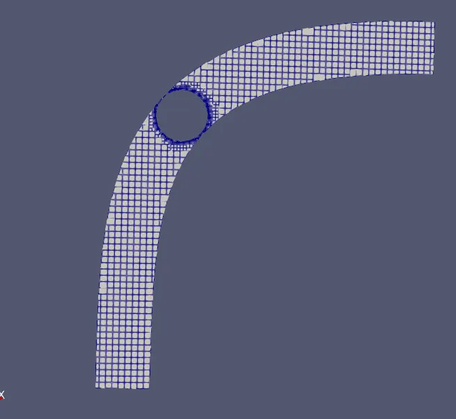
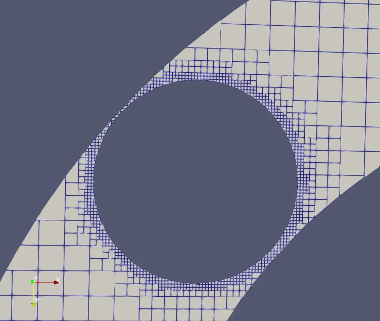
the basic mesh size:
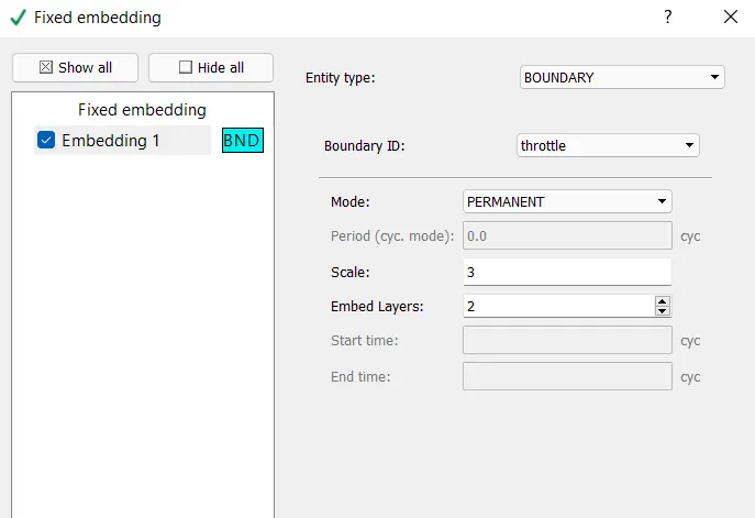
mesh scale for throttle are specifies :
After that specified case setup file are exported to folder and run simulation.
The simulation for number of cycle are run in cygwin command window.
Post convert the file that is simulated in cygwin command and file name is given.
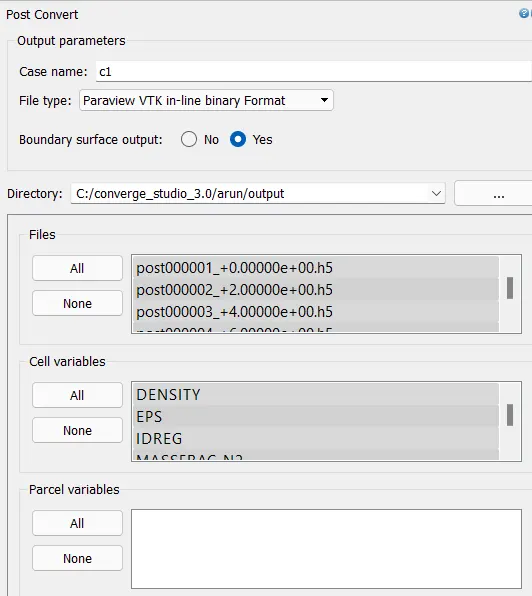
As the simulation is binary files called post file are generated inside the output folder. these files have an extension *.out. now these files are written by CONVERGE. these files contain information regarding the 3D flow field. We use a special software called paraview that can read this flow information. However before paraview can do this the file have to be converted to a form taht paraview can understand. These is done using a tool called post convert. ater the conversion we load the files into paraview.
RESULTS:
MESH:
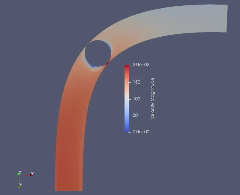
velocity contour:
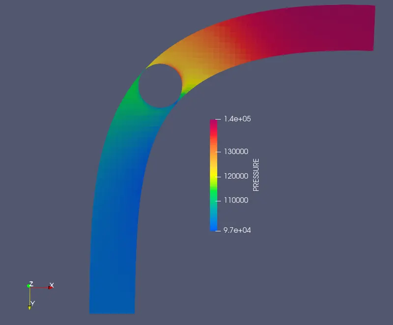
pressure contour:
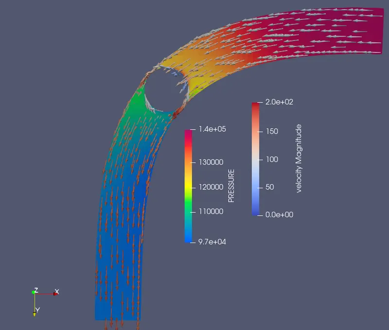
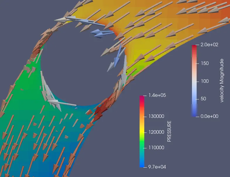
vector lines:
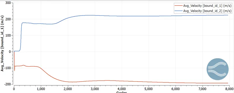
velocity plots:
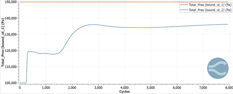
pressure plots:
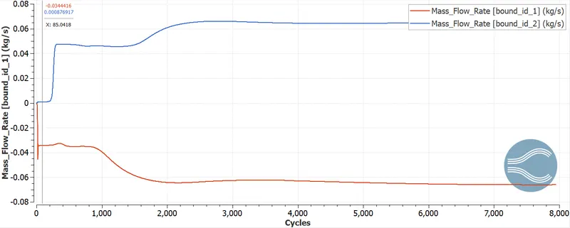
mass flow rate:
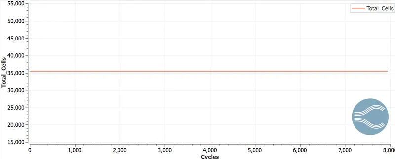
total cell:
animation link:
CONCLUSION:
* In velocity contour it can be seen that the velocity of the fluid reazhs zero near the throttle value due to obstruction. this point where the fluid velocity reaches xero is called as syagnation point. as the fluid passes through the throttle valve the velocity of the fluid increases.
* In the velocity plot it can be seen that fluid velocity increases as it flows from inlet to outlet. this is due to increase in the flow area.
* In the pressure contour it can be seen that the fluid experience high pressure near the wall of the throttle valve this is because the fluid velocity is zero near the throttle valve walls.
* In the total pressure plot it can seen that the total pressure in constant at inlet due to boundary conditions and increases at outlet due to increase in fluid velocity which further increases dynamic pressure.