Week 4.1 - Genetic Algorithm

* GENETIC ALGORITHM

A genetic algoritham (GA) is used to solve both constrain and un constrained optimization problems based on natural selection proces that minize the biological evalution.

at each step the genetic algoritham randomly select individuals from current population and uses them as a parents to produce children for next generation . over succesive generations the population evolves towards an optimal solution.

it basicaly use three main type of rules..... selection, crosscover, mutation

Genetic algoritham(ga)syntax

1 x=ga(@func,nvar)

where func is a function and nnvar is the number of variable

2 x=ga(2func,nvar,A,B,Aeq,Beq)

set of lower bond and upper bond is given so the solution lies in range.

3 x=ga(@func,nvars,A,B,Aeq,Beq,lb,ub,nonlcon,intcon,options)

A,B=linear inequality constraints

Aeq,Beq= linear equality constraints

lb=lower bond

up=upper bond

nonlcon=non linear constraints

intcon=vector of positive integers

options= optimization options

* PROGRAM FOR FUNCTION STALAGMITE

% equation of stalagmite.

function f=stalagmite(input_vector)
          x=input_vector(1);
          y=input_vector(2);
      
     f1=(sin(5.1*pi*x+0.5))^6;
     f2=(sin(5.1*pi*y+0.5))^6;
     f3=exp((-4*log(2)*(x-0.0667)^2)/0.64);
     f4=exp((-4*log(2)*(y-0.0667)^2)/0.64);

     f=-(f1*f2*f3*f4);

end

* PROGRAM FOR FINDING GLOBAL MAXIMA.

clear all
close all
clc

%defining our stage space
x=linspace(0,1,150);
y=linspace(0,1,150);

num_case=50;

[X,Y]=meshgrid(x,y)

% evaluating the stalagmite equation
for i=1:length(X)
   for j=1:length(Y)
    input_vector(1)=X(i,j);
    input_vector(2)=Y(i,j);
    f(i,j)=stalagmite(input_vector);
   end
end

surfc(X,Y,f);
xlabel('X axis')
ylabel('Y axis')
shading interp

tic
% study_time 1

for i=1:num_case
    [inputs,fopt(i)]=ga(@stalagmite,2);
    xopt(i)=inputs(1);
    yopt(i)=inputs(2);

end
study1_time=toc;

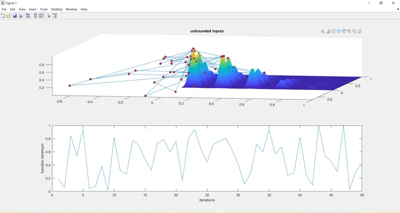
figure(1)
subplot(2,1,1)
hold on
surfc(x,y,-f)
shading interp
plot3(xopt,yopt,-fopt,'Marker','o','MarkerSize',6,'MarkerFaceColor','r')
title('unbounded inputs')
subplot(2,1,2)
plot(-fopt)
xlabel('iterations');
ylabel('function minimum');

tic
%study2_time

for i=1:num_case
    [inputs,fopt(i)]=ga(@stalagmite,2,[],[],[],[],[0;0],[1;1]);
    xopt(i)=inputs(1);
    yopt(i)=inputs(2);
end
study2_time=toc;

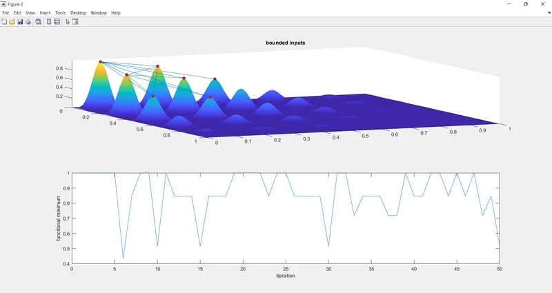
figure(2)
subplot(2,1,1)
hold on
surfc(x,y,-f)
shading interp
plot3(xopt,yopt,-fopt,'Marker','o','MarkerSize',6,'MarkerFaceColor','r')
title('bounded inputs')
subplot(2,1,2)
plot(-fopt)
xlabel('iteration');
ylabel('functional minimum');


% increasing ga iteration
options=optimoptions('ga')
options=optimoptions(options,'PopulationSize',300);

tic
for i=1:num_case
    [inputs,fopt(i)]=ga(@stalagmite,2,[],[],[],[],[0;0],[1;1],[],options);
    xopt(i)=inputs(1);
    yopt(i)=inputs(2);
end

study3_time=toc

figure(3)
subplot(2,1,1)
hold on
surfc(x,y,-f)
shading interp
plot3(xopt,yopt,-fopt,'Marker','o','MarkerSize',6,'MarkerFaceColor','r')
title('bounded inputs with modified popukation size')
subplot(2,1,2)
plot(-fopt)
xlabel('iteration')
ylabel('function minimum')

OUTPUTS

STUDY 1

STUDY 2

STUDY 3

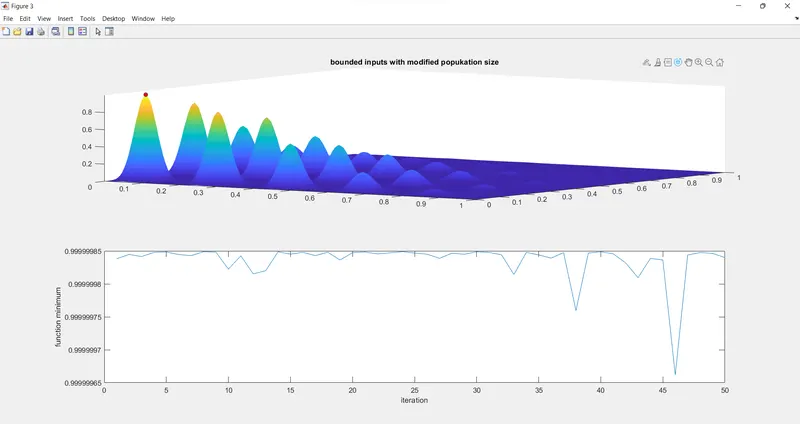
Peak point is called global maxima.

in matlab ......ga calculates the global minima in order to show global maxima we add -ve to 'f' and 'fopt' everywhere.