Week 8: Literature review - RANS derivation and analysis

INTRODUCTION:

TYPES OF FLUID FLOW

Fluid can be split into three types-

-laminar flow

-transient flow

-turbulrnce flow

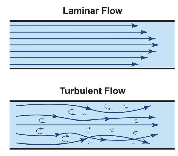
The type of flow can be determined by using the rynolds number. a low reynolds corresponds to laminar flow where the flow is in an orderly manner and parametrs like pressure and velocity remain steady. a high reynolds number corresponds to turbulent flow where the flow is chaotic and the parameters are fluctuating.

Theory of turbulemce:

Turbulence is an unstedy, irregular motion in which transport quantites(mass, momentum, sclar spicies) flucates in space and time. it is contrast to laminar flow, which occurs when a fluid flows in parallel layers with no disruption between those layer. Turbulence is caused by excessive kinetic energy in parts of fluid flow, which overcomes the damping effects of the fluid viscosity. for this reason turbulence is commonly realized in low viscosity fluids.

Turbulence modelling:

Turbulence modelling is used to calculate reynolds stress and turbulent viscosity. the effect of turbulence an be modelled using a method called as direct numerical simulation. which involves in solving navies strokes equation over turbulent time step. but the turbulent time step is very samll thus computational cell size is required to solve. therefore turbulence model is used to capture the effect of turbulence in coarse grid size.

basically three different turbulence models are used:

-reynolds averaged navier stroke equation(RANS)

-large eddy simulation (LES)

-direct numerical simulation(DNS)

The aim here is to derive reynolds stress expression by performing reynolds decomposition on the NS equation if we take any standard book on boundary layer theory we see that the following equation are valid. the below derivation is derived for 2 dimensional equation. equation that govern the boundary layer are-

continuity equation

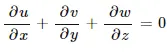
momentum equation along x-direction

All the above equation are valid inside the boundary layer we see that some of the term are missing because inside the boundary layer we can neglect some terms based upon the order of magnitude analysis. in this case we will a final set of equation which we can siimulate boundary layer on any type of geometry.

But so far we have used only turbulence model. so whenevr we simulate a shock flow problem or a conjugate problem we use a turnulent model. if we solve the above 3 equation it is completely capable of giving solution for laminar and turbulaent problems by doing that we can say that we are performing the direct numaerical analysis

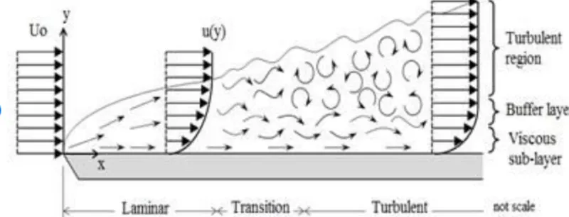
Here in the above image shown if we take a velocity probe and put it in the turbulent region to measure the velocity as a functional of time then we get a profile like this

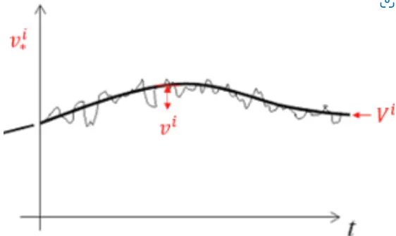
here the velocity cariation is continously fluctuating and if we measure the frequency of fluctuation and inverse it we can calculate something called as turbulent time step and this step is very samll and it occurs for a small distance. so if by taking the governing equation and integrating it over that small time step and is we have a high number of compulational simulations and that is why we use turbulence model so that we can still capture of turbulence by using a courser grid and a large time step.

Now we are going to take the governing equation and interval it over atime which is much larger then the turbulent time sacle so this is called the averaging process. Then we apply the reynolds decomposition and convert this original set of equation into a form called as reynold average navier strokes equation(RANS)

We than use this equation along with the turbulent model to simulate the turbulent flow, in this process we end up with some unknown terms which have to be modelled. The first step is to split the velocity component or any other flow variable into the mean component and a fluctuating component this is called the reynold decomposition.

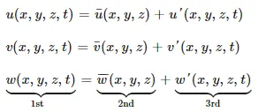
1st is the instantenous velocity at any space and time

2nd is the mean component function of space and 3rd is the fluctuating component function of time and space

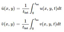
here after integrating the velocity component we get the averaged velocity which is independent of time another intresting property is that when we integrating the fluctuations its always going to be zero let us drive why this is the case

this is reynolds decomposition and let us say that i time average this

now the 2nd term in this the averaged quantity now if we time average the averaged quantity we get an averaged quantity

so,

So here rhe 3rd term which is fluctuating term will become zero. so the idea is when we integrate for a longer time step the fluctuation tends to become zero, and this rule can be applied to other quantities as well.

now applying this integral rule to the continuity equation

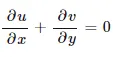
applying decompostion

integrating the above time

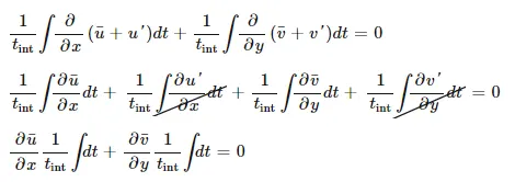
now applying the limts to integration

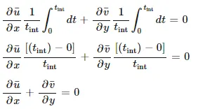
so the time averaged velocity component satisfy the contunity equation

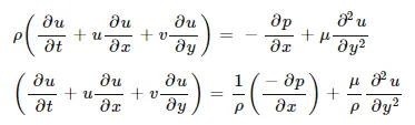
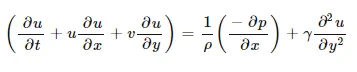
replacing as kinetic viscosity

now on LHS we will add a term that is x component of velocity multiplied by the continuity equation we are doing this to convert the above equation to a much more suitable form.

the underlined term in the above equation is =0 so it dosent change anything now rearranging the terms

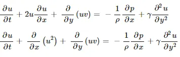
now we are ready to apply the time integration and aslo the reynold decomposition

now wxpanding the equation

now cleaning the equation a bit we get

so here the initial terms are same as that of momentum equation the difference is that they were instantaneous quantities and they are time averaged.

now we will make an assumption in the boundary layer the layer is very small especially when you compare it to the plate the argument that we can make is the gradient in the velocity component are going to be much more stronger in the y direction compare to the x direction because in that small space yhe value for the velocity component changes a lot anlog the y axis, but along the x axis it changes are not that much and hence we are going to neglect it

neglecting this in the RHS

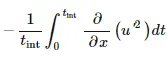
this is true only inside a boundary layer

so the RHS of the equation becomes

now here the below term is molecular viscosity term

and below term is momentum diffusity of turbulence

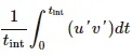
now here we can say that diffusion of momentum takes place in 2 ways 1 is through molecular viscosity and the other is through turbulence motion.