To Plot Pv Diagram For Otto Cycle & Calculate The thermal Efficiency Of Otto Cycle By Using Mat-lab.

Aim:-To Plotting Pv Diagram For Otto Cycle And Calculating The thermal Efficiency Of Otto Cycle By Using Mat-lab.

Theory:-An Otto Cycle Is An Idealized Thermodynamic Cycle That Describes The Functioning Of a Typical Spark Ignition Piston Engine.It Is The Thermodynamic Cycle Most Commonly Found In Automobile Engines

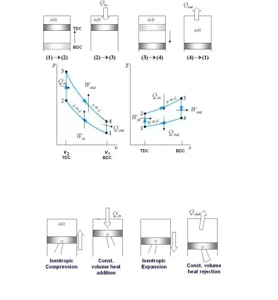
The Otto cycle 1 → 2 → 3 → 4 consists of following four processes:

Process 1 → 2: Reversible adiabatic compression of air;

Process 2 → 3: Heat addition at constant volume;

Process 3 → 4: Reversible adiabatic expansion of air;

Process 4 → 1: Heat rejection at constant volume.

Code:-

clear all
close all
clc
%input
gamma=1.4;
t3=2500;

%state variable 
p1=101325;
t1=500;
%engine geomatric perameters 
bore=0.1;
stroke=0.1;
connecting_rod=0.15;
cr=12;

%calculate the swept volume and clerance volume
v_swept=(pi/4)*bore^2*stroke;
v_clerance=v_swept/(cr-1);
v1=v_swept+v_clerance;
v2=v_clerance;

% state variable at point2
p2=p1*(v1/v2)^gamma;
constant_c=p1*v1^gamma; 

t2=(p2*v2*t1)/(p1*v1);
v_compression=engine_kinamatic(bore,stroke,connecting_rod,cr,180,0);
p_compression=constant_c./v_compression.^gamma;
% state variable at point 3
v3=v2;

p3=p2*t3/t2;
constant_c=p3*v3^gamma;
v_expension=engine_kinamatic(bore,stroke,connecting_rod,cr,0,180);

p_expension=constant_c./v_expension.^gamma;
%state variable at point4
v4=v1;
p4=p3*(v3/v4)^gamma;

n = 1 - 1/(cr^gamma-1);


%plotting
figure(1)
hold on 
plot(v1,p1,'*','color','b')
plot(v2,p2,'*','color','b')
plot(v3,p3,'*','color','b')
plot(v4,p4,'*','color','b')
grid on

plot(v_compression,p_compression)
plot(v_expension,p_expension)
plot([v2 v3], [p2 p3],'color','g')
plot([v4 v1], [p4 p1],'color','g')
xlabel('(volume)')
ylabel('(pressure)')
title('(Otto Cycle)','fontsize',21)
text(v1,p1,'state-1','fontsize',8)
text(v2,p2,'state-2','fontsize',8)
text(v3,p3,'state-3','fontsize',8)
text(v4,p4,'state-4','fontsize',8)

text(3*10^(-4),3*10^6,[sprintf('Thermal Efficieny=%d',n)])

Procedure:-

Following Steps Used To Plot Pv Diagram And Calculate Efficiency Of Otto Cycle In Mat-lab .

• Creating New File ,Inputs Are Initialized.

P1=101325 , T1=500,T3=2500 ,Cr=12,(Gamma)=1.4

• Swept Volume And Clearance Volume Are Calculated By Using Following Formulas

V_Swept =(Pi/4)*Bore*Stroke

V_Clearance=V_Swept/(Cr-1)

• Remaining Variable Are Calculate Based On Following Relation:-

For Constant Volume Process V2=V3 V4=V1

For Isentropic Compression P1*(V1^Gamma)=P2*(V2^Gamma)

For Isentropic Expansion P3*(V3^Gamma)=P4*(V4^Gamma)

Pv/T=Constant

• Plot Command Is Used To Plot (V1 P1),(V2 P2),(V3 P3),(V4 P4) Points On Graph.
• Same Plot Command Can Be Used To Plot Straight Line In Graph Using Points, But To Creat The Curves Vector Points Are Needed.
• To Creat Vector Points A Function Is Created

function [v] = engine_kinamatic(bore,stroke,connecting_rod,cr,start_crank,end_crank)

a=stroke/2;
R=connecting_rod/a;
v_s=pi/4*bore^2*stroke;
v_c=v_s/(cr-1);

theta =linspace(start_crank,end_crank,100);

term1=0.5*(cr-1);
term2=R+1-cosd(theta);
term3=(R^2-sind(theta).^2).^0.5;

v=(1+term1*(term2-term3)).*v_c;


end
​

• The Function Takes Engine Parameters (Bore,Stroke, Connecting_Rod,Compression Ratio),Initial And Final Piston Angle As Input And Gives A Vector Variable As Output.
• Function Output Is Saved As Compression Volume Vector Variable And Compression Pressure Is Calculated Using Equation

P*(V^Gamma)=Constant

• This Creates Array Of Volume And Pressure Point Along Compression Curve, To Plot Compression Curve .
• Same Will Be Repeated For Isentropic Expansion Curve.
• Thermal Efficiency Is Calculated By Using Formula

Efficiency(N)=1-(1/Cr(Gamma-1)

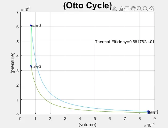
OUTPUT:-

THERMAL EFFICIENCY=9.68176e-01