Genetic Algorithm

Aim:-To Write Code in mat-lab to optimize the stalagmite and find global maxima of the function.

Theory:-

Genetic Algorithm:- Is a Method For Solving Both Constrained And Unconstrained Optimization Problems That Is Based On Natural Selection, The Process That Drives Biological Evolution. The Genetic Algorithm Repeatedly Modifies a Population Of Individual Solutions. At Each Step, The Genetic Algorithm Selects Individuals At Random From The Current Population To Be Parents And Uses Them To Produce The Children For The Next Generation. Over Successive Generations, The Population "Evolves" Toward An Optimal Solution. You Can Apply The Genetic Algorithm To Solve a Variety Of Optimization Problems That Are Not Well Suited For Standard Optimization Algorithms, Including Problems In Which The Objective Function Is Discontinuous, Non Differentiable, Stochastic, Or Highly Nonlinear. The Genetic Algorithm Can Address Problems Of Mixed Integer Programming, Where Some Components Are Restricted To Be Integer-Valued.

The Genetic Algorithm Uses Three Main Types Of Rules At Each Step To Create The Next Generation From The Current Population:

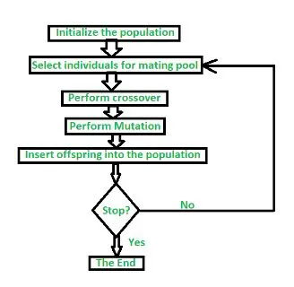
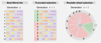
Selection Rules :-It Select The Individuals, Called Parents, That Contribute To The Population At The Next Generation.In This Step , The Parents Are Selected From The Sample Data Points, The Main Objective Of The Selection Process Is To Select The Highly Fit Individuals.

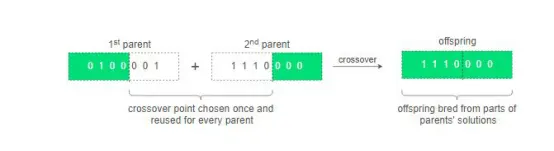
Crossover Rules:- It Is The Process Of Two Parents Solutions And Producing The Child From Them.There Are Many Ways To Do Cross- Over Operations(Combine Two Parents To Form Children For The Next Generation.)

Example :-one point cross over method ,where set of genes from parents a is combined with parents b to create a new offspring.

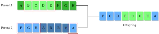
Mutation Rules :-Mutation Is Carried Out To Maintain The Genetic Diversity From One Generation Of Chromosome To The Next .If Mutation Is Not Performed, The Chromosome Will Become Too Similar To Each Other , Converge Takes Place Soon And The Result In Local Minim.(Apply Random Changes To Individual Parents To Form Children)

Application of ga:- Genetic Algorithm Are Mainly Used In optimization problems of various kinds, they are frequently used in various application area as well.

• Optimasition-GeneticAlgorithm Are most commonly used in optimization problems

Where in we have maximize or minimize a given objective function value a given set of conditions

• Netural network :-ga are also used to train netural networks, particularly recurrent netural networks
• Image processing :-ga are also used for various digital image processing (dip) tasks as well like dense pixel machining.

Syntax Of ga:- ga is used to the minimum function.

X=ga (Fun, Nvars ,a , b, Aeq , Beq , 1b,ub,non1con, Options)

Use the geomatric algorithm to minimize the ps_example function on the region x(1)+x(2)==5+(1) using a constrain tolerance that is smaller than the default

First, convert the two constrains to matrix from A*x<=b and Aeq*x =beq.in other words, get the variable on the left hand side of the expression, and make the inequality into less then or equal form

-x(1)-x(2)<=-1

-x(1)+x(2)==5

A=[-1,-1]

b=-1

Aeq=[-1,1];

Beq=5;

To obtain more accurate solution ,set a constrain tolerance of 1e-6.and to moniter the solver process, set a plot function.

Options=optimations(‘ga’,’constrain tolerance’,’1e-6’,’plotfcn’, @gaplotbestf);

Solve the minimization problem.

rng default %free reproducibility

Fun=@ps_example;

X=ga(fun,2, A,b,Aeq ,Beq,[],[],[],options)

Input arguments:-

• Fun:-Objective function, specified as a function handle or function name. Write the objective function to accept a row vector of length nvresand return a scalar value.

When the 'UseVectorized' option is true, write fun to accept a pop-by-nvars matrix, where pop is the current population size. In this case, fun returns a vector the same length as pop containing the fitness function values. Ensure that fun does not assume any particular size for pop, since ga can pass a single member of a population even in a vectorized calculation.

Example: fun = @(x)(x-[4,2]).^2

Data Types: char | function_handle | string

• Nvres:-Number of variables, specified as a positive integer. The solver passes row vectors of length nvarsto fun.

Example: 4

Data Types: double

• A— Linear inequality constraints:-

Linear inequality constraints, specified as a real matrix. A is an M-by-nvars matrix, where M is the number of inequalities.

A encodes the M linear inequalities

A*x <= b,

where x is the column vector of nvars variables x(:), and b is a column vector with M elements.

For example, to specify

x1 + 2x2 ≤ 10
3x1 + 4x2 ≤ 20
5x1 + 6x2 ≤ 30,

give these constraints:

A = [1,2;3,4;5,6];

b = [10;20;30];

Example: To specify that the control variables sum to 1 or less, give the constraints A = ones(1,N) and b = 1.

Data Types: double

• b— Linear inequality constraints:-

Linear inequality constraints, specified as a real vector. b is an M-element vector related to the A matrix. If you pass b as a row vector, solvers internally convert b to the column vector b(:).

b encodes the M linear inequalities

A*x <= b,

where x is the column vector of N variables x(:), and A is a matrix of size M-by-N.

For example, to specify

x1 + 2x2 ≤ 10
3x1 + 4x2 ≤ 20
5x1 + 6x2 ≤ 30,

give these constraints:

A = [1,2;3,4;5,6];

b = [10;20;30];

Example: To specify that the control variables sum to 1 or less, give the constraints A = ones(1,N) and b = 1.

Data Types: double

Aeq — Linear equality constraints:-

Linear equality constraints, specified as a real matrix. Aeq is an Me-by-nvars matrix, where Me is the number of equalities.

Aeq encodes the Me linear equalities

Aeq*x = beq,

where x is the column vector of N variables x(:), and beq is a column vector with Me elements.

For example, to specify

x1 + 2x2 + 3x3 = 10
2x1 + 4x2 + x3 = 20,

give these constraints:

Aeq = [1,2,3;2,4,1];

beq = [10;20];

Example: To specify that the control variables sum to 1, give the constraints Aeq = ones(1,N) and beq = 1.

Data Types: double

• beq— Linear equality constraints

Linear equality constraints, specified as a real vector. beq is an Me-element vector related to the Aeq matrix. If you pass beq as a row vector, solvers internally convert beq to the column vector beq(:).

beq encodes the Me linear equalities

Aeq*x = beq,

where x is the column vector of N variables x(:), and Aeq is a matrix of size Meq-by-N.

For example, to specify

x1 + 2x2 + 3x3 = 10
2x1 + 4x2 + x3 = 20,

give these constraints:

Aeq = [1,2,3;2,4,1];

beq = [10;20];

Example: To specify that the control variables sum to 1, give the constraints Aeq = ones(1,N) and beq = 1.

Data Types: double

• lb— Lower bounds:-Lower bounds, specified as a real vector or array of doubles. lb represents the lower bounds element-wise in lb ≤ x ≤ ub.

Internally, ga converts an array lb to the vector lb(:).

Example: lb = [0;-Inf;4] means x(1) ≥ 0, x(3) ≥ 4.

Data Types: double

• ub— Upper bounds:-

Upper bounds, specified as a real vector or array of doubles. ub represents the upper bounds element-wise in lb ≤ x ≤ ub.

Internally, ga converts an array ub to the vector ub(:).

Example: ub = [Inf;4;10] means x(2) ≤ 4, x(3) ≤ 10.

Data Types: double

nonlcon — Nonlinear constraints:-
Nonlinear constraints, specified as a function handle or function name. nonlcon is a function that accepts a vector or array x and returns two arrays, c(x) and ceq(x).

c(x) is the array of nonlinear inequality constraints at x. ga attempts to satisfy

c(x) <= 0

for all entries of c.

ceq(x) is the array of nonlinear equality constraints at x. ga attempts to satisfy

ceq(x) = 0

for all entries of ceq.

For example,

x = ga(@myfun,4,A,b,Aeq,beq,lb,ub,@mycon)

where mycon is a MATLAB® function such as

function [c,ceq] = mycon(x)

c = ... % Compute nonlinear inequalities at x.

ceq = ... % Compute nonlinear equalities at x.

options — Optimization options:-

Optimization options, specified as the output of optimoptions or a structure.

optimoptions hides the options listed in italics. See option that optimised the hide Values in {} denote the default value.

{}* represents the default when there are linear constraints, and for MutationFcn also when there are bounds.

I* indicates that ga handles options for integer constraints differently; this notation does not apply to gamultiobj.

NM indicates that the option does not apply to gamultiobj.

Example: optimoptions('ga','PlotFcn',@gaplotbestf)

IntCon — Integer variables

Integer variables, specified as a vector of positive integers taking values from 1 to nvars Each value in IntCon represents an x component that is integer-valued.

Example: To specify that the even entries in x are integer-valued, set IntCon to 2:2:nvars

Data Types: double

Mat-lab code:-

step 1:- In step1 we gave input to the for loop by num_cases.according to that the for loop will repeat operations and generate the random data .

clear all 
close all
clc

%defining our search space 

x=linspace(0,0.6,150);
y=linspace(0,0.6,150);
num_cases=50;

%creating a 2d dimensional mesh 
[xx,yy]=meshgrid(x,y);

%evaluating the stalagmite function
for i=1:length(xx)
    for j=1:length(yy)
        inputvector(1)=xx(i,j);
        inputvector(2)=yy(i,j);
        f(i,j)=stalagmite(inputvector);
    end 
end


%study 1-statical behaviour
tic

for i=1:num_cases
    [input,fopt(i)]=ga(@stalagmite,2);
    xopt(i)=input(1);
    yopt(i)=input(2);
end

Study1_time = toc;
figure(1)
subplot(2,1,1)
xlabel('xaxis')
ylabel('yaxis')
hold on
surfc(xx,yy,-f)
shading interp
plot3(xopt,yopt,-fopt,'marker','o','markersize',5,'markerfacecolor','r')
title('unbounded inputs')
subplot(2,1,2)
plot(-fopt)

xlabel('iteration')
ylabel('function minimum')


%calling stalagmite function

function [f]= stalagmite(inputvector)
x=inputvector(1);
y=inputvector(2);
f1x=(sin(5.1*pi*x+0.5)).^6;
f1y=(sin(5.1*pi*y+0.5)).^6;


f2x=exp(((-4)*log(2)*(x-0.0667)^2)/(0.64));
f2y=exp(((-4)*log(2)*(y-0.0667)^2)/(0.64));

f= -(f1x*f1y*f2x*f2y); 


end 

Output1:-

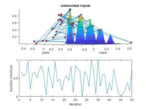
step2:-In step2 we will gave boundery conditions to the data .after analysing this boundary conditions the ga will gave local maxima with in the given range.

%study 2-statical behaviour with uppper and lower bonds

tic
for i=1:num_cases
    [input, fopt(i)]=ga(@stalagmite,2,[],[],[],[],[0;0],[1;1]);
    xopt(i)=input(1);
    yopt(i)=input(2);
end

Study2_time = toc
figure(2)
subplot(2,1,1)
xlabel('xaxis')
ylabel('yaxis')

hold on
surfc(x,y,-f)
shading interp
plot3(xopt,yopt,-fopt,'marker','o','markersize',5,'markerfacecolor','r')
title('bounded inputs')
subplot(2,1,2)
plot(-fopt)
xlabel('iteration')
ylabel('function minimum')

Output2:-

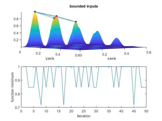
step3:-In step3 firstly we will optimise the ga with the inbuilt command "optimations "

In optimations we will increses the value of data range so ,that we will get the global maxima.

%study 3-statical behaviour with uppper and lower bonds

options=optimoptions('ga');
options=optimoptions(options,'populationsize',170);

tic
for i=1:num_cases
    [input, fopt(i)]=ga(@stalagmite,2,[],[],[],[],[0;0],[0.6,0.6],[],[],options);
    xopt(i)=input(1);
    yopt(i)=input(2);
end

Study3_time = toc
figure(3)
subplot(2,1,1)
xlabel('xaxis')
ylabel('yaxis')
hold on
surfc(x,y,-f)
shading interp
plot3(xopt,yopt,-fopt,'marker','o','markersize',5,'markerfacecolor','r')
title('bounded inputs')
subplot(2,1,2)
plot(-fopt)
xlabel('iteration')
ylabel('function minimum')

Output3:-

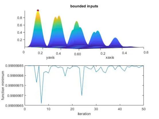
Stopping criteria:-the optimisation stopped when it completed the one iteration cycle and after completing the cycle the optimisations get’s terminated (stopped) .

Significance of running multiple iteration and causes:-

In The Program I have Used Num_Cases Which Is a Variable.By the help of this variable we will give input to the program which is inside the for loop.and the repetation of for loop cycle is depends upon the num_cases value.

Example -if we give 40 value to the num_cases that’s means the for loop will repeat the program for 40 times.