Solving second order ODEs

Aim:-

To Write a Program In Mat-Lab That Will Simulate The Pendulum Motion.

Objective:-

The Objective Of The Program Is To Simulate The Motion Of Pendulum With Give Values.

Gravity g=9.81(m/s)

Length Of Pendulum l=1(m)

Mass of ball =1(kg )

Damping coefficient,b=0.05(kg/s)

Total Duration t=20(s)

Initial Condition At t=0(s)

Angular Displacement θ=0(rad)

Angular_Velocity θ=3(Rad/s2)

Theory:-

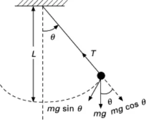
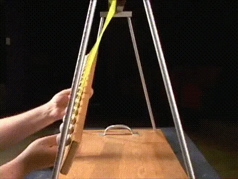
A Pendulum Is a Weight Suspended Form Pivot At One End So That It Can Swing Freely.When a Pendulum Is Displaced From Its Rest Position It Is Subjected To Resisting Force Of Gravity That Will Accelerate It Back Towards The Equilibrium Position.When Released, The Restoring Force Acting On The Pendulum Mass Causes It To Oscillate About Its Equilibrium Position Swing Back And Forth.The Time To Complete One Cycle From Left Swing To Right Swing Is Called Period It Depends On The Length Of The Pendulum, Width & The Pendulum Swing.

Mat-Lab Solver ODE45 :-

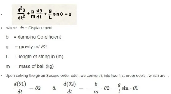
In Order To Solve The Above Reduced ODE,We Require The Time Span And Initial Conditions.

The Reduce Ode Ca Be Solved In Mat-Lab Using Inbuilt Ode Solver, Ode45 Whose Syntax Is Shown In Below:

[t,y] = Ode45(odefun,tspan,y0)

The Above Syntax Integrates the system of differential equation y’=f(t,y) from t_initial to t_final,

I.e. t_span with initial conditions,i.e.y thus, giving output as t and y. here ,y represent the angular displacement , θ which is needed to transform in to coordinates system in order to plot over a plane and visualize the motion .

Mat-lab Code:-

clear all 
close all 
clc

b=0.05;
g=9.81;
l=1;
m=1;

%inital conditions 
theta_0=[0;3];
%time points
t_span=linspace(0,20,500);

%solve ode
[t,results]= ode45(@(t,theta)ode_func(t,theta,b,g,l,m),t_span,theta_0);
%plotting
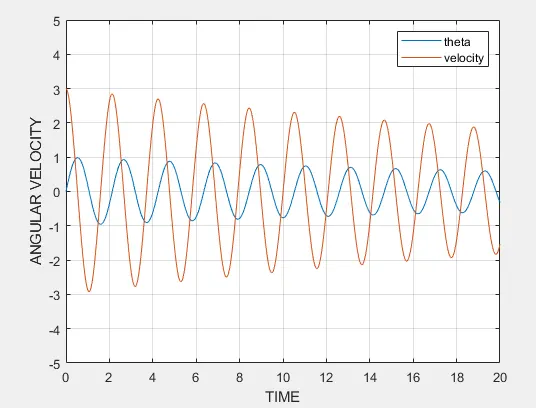
figure(1)
plot(t,results(:,1))
hold on 
plot(t,results(:,2))
axis([0 20 -5 5])
xlabel('TIME')
ylabel('ANGULAR VELOCITY')
legend('theta','velocity');
grid on
ct=1;
for i=1:length(results(:,1))
    x0=0;   %fix point
    y0=0;   %fix point
    l=1;
    x1=l*sin(results(i,1));
    y1=-l*cos(results(i,1));
    
    figure(2)
    
    plot([-1 1],[0 0],'linewidth',5,'color','b');
    hold on
    
    plot([x0 x1],[y0 y1],'linewidth',3,'color','g');
    hold on
    
    plot(x1,y1,'o','markersize',20,'markerfacecolor','r');
    grid on
    axis([-2 2 -2 2]);
    pause(0.03);
    hold off;
    M(ct)=getframe(gcf);
    ct=ct+1;
   
end 
    movie(M)
    videofile = VideoWriter('pendulam_simulation.avi','uncompressed AVI');
    open(videofile)
    writeVideo(videofile,M)
    close(videofile)
    
    
 

Function command:-

function [dtheta_dt]=ode_func(t,theta,b,g,l,m)
theta1=theta(1);
theta2=theta(2);
dtheta1_dt=theta2;
dtheta2_dt= -(b/m)*theta2-(g/l)*sin(theta1);
dtheta_dt=[dtheta1_dt;dtheta2_dt];
end

Output:-

video link :-

https://drive.google.com/file/d/1JqXNzyTi3xC_3NWSOgu87Hiy7eTDrNgf/view?usp=sharin