WOT(Wide open Throttle)

Aim:-1.To Evaluate The Hill Climbing Ratio Of Tata Ultra-Truck At Fully Loaded Conditions.

2.Analyse The Grade-Ability And Its Associated Parameters.

3.Analyse The Force Acting On The Vehicle By Creating a Drive Cycle And Plot Graph Of Speed Vs Time.
4.Modeling Of Wot (Wide Open Throttle)Of Gm Ev1 Car And Compare The Data With 5% Charge In Parameters To Original Dataset.

Solution1:-

Ratio Of Hill Climbing Power Required By Fully Loaded And Half Loaded Tata Ultra Truck.

We Are Taking The Parameter Of TATA ULTRA T10 TRUCK For Hill Climbing Power Ratio.

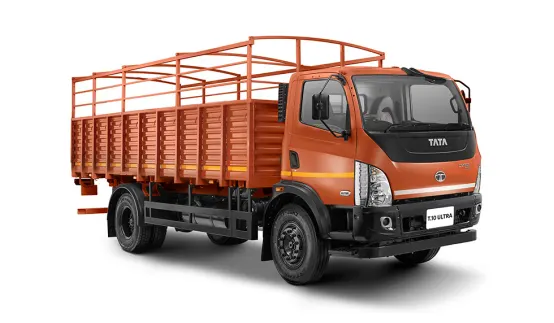
Data Extracted:-

Gross weight-9600kg

Payload-6350kg

Kerb weight-3250kg

Gradebility-30%(0.3)

Assumption

the truck is climbing the hill at a constant speed of 40kmph(11.1m/s).

To find:-

Hill climbing power ratio=?

G=(rise/run)*100%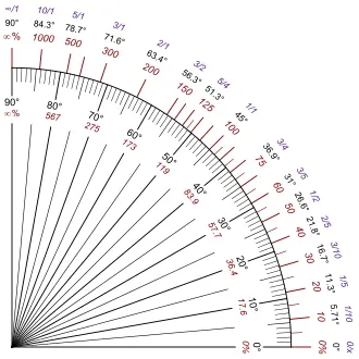

G=(tan `theta`)

G=tan^-1 (0.3)

G=16.7`degree`

Fully loaded conditions,

Gross weight= kerb weight+payload

Gross weight= 3250+6350

Gross weight=9600kg

Hill climbing force

`F_hc=m.g.sin`fyi``

`F_hc=9600*9.81*sin(16.7)

`F_hc(FULL-LOAD)=27062.46 N`

Hill climbing Power

`P_hc(FULL-LOAD)=F_hc*v`

`P_hc(FULL-LOAD)=27062.46*11.1`

`P_hc(FULL-LOAD)=300.39 KW`

Half loaded condition

For half loaded the payload of the vehicle should be reduced to half the value.

Payload=6350/2=3175kg

Hill climbing force

`F_hc=m.g.sin`psi``

`F_hc=6425*9.81sin(16.7)`

`F_hc=17648.19N

Hill climbing Power

`P_hc(HALF-LOADED)=F_hc*v`

`P_hc(HALF-LOADED)=17648.19*11.1`

`P_hc(HALF-LOADED)=195.89 kw`

Hill climbing power ratio

`POWER RATIO=frac{P_hc(FULL-LOAD)}{P_hc(HALF-LOADED)}`

`POWER RATIO=frac{300.39}{195.89}

`POWER RATIO=1.6

Solution2:- GREADIBILITY AND IT’S PERIMETER

Given

minimum height (RISE)=5.5m

To find minimum length of the flyover=?

We are assuming the grade-ability (angle)=16.7`degree`(FROM TATA ULTRA TRUCK)

`tan psi =frac{RISE}{RUN}`

`RUN =frac{5.5}{tan (16.7)}

`RUN=18.33m`

NOW,

`Sin psi=frac{Rise}{L(hypotenuse)}`

`L(hypotenuse)=frac{5.5}{Sin 16.7}`

`L(hypotenuse)=19.6m

VERIFICATION OF THE CALCULATION

`GREADIBILITY=frac{RISE}{RUN}*100%`

`GREADIBILITY=frac{5.5}{18.33}*100%`

`GREADIBILITY=30%`

RESULT:- The Minimum Length Of The Flyover Is 19.6M

Solution3:- PREPARING A DRIVE CYCLE AND PLOT GRAPH OF TIME VS VELOCITY USING SIMULINK.

In this analysis, we are taking the Simulink model from the MathWorks website and feeding our drive cycle to plot time vs velocity graph.

MODEL:-

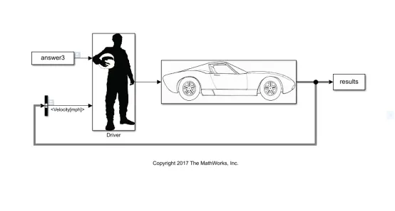
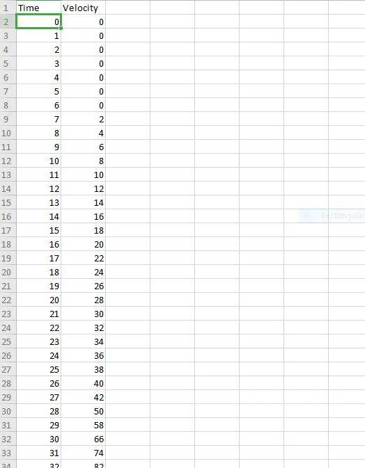
• l The Drive Cycle data will be fed to the from workspace block.
• l From the from workspace block the velocity data will be sent to the driver block and compared to the calculated velocity to determine any error.
• l After checking the error in the data will be fed into the glider block for calculations and output to be sent to the results block.

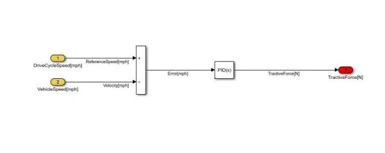
DRIVER MODEL:-

• PID – Proportional, Integrate, and Differential block where it checks the error so that there is no exceeding difference in the default value.
• Then we get the desired output if the condition gets satisfied in the PID block.
• The output we are obtaining as Tractive Force (`F_te`).

GLIDER MODEL:-

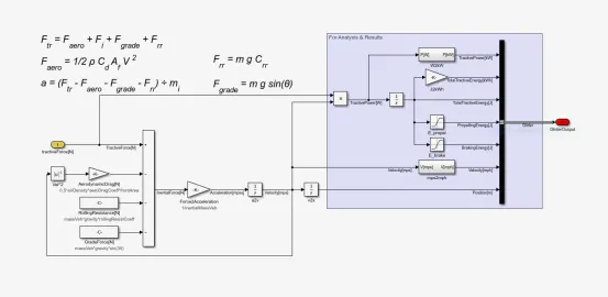
om the driver module we take the output and give it as input in the glider model.

Where the Traction force is a sum of drag, hill climbing, inertia, rolling resistance,

` F_te=F_rr+F_ad+F_hc+F_i`

` F_te=F_rr+F_ad+F_hc+F_i`

From this, the inertia force is being calculated,

` F_i=F_te–(F_rr+F_ad+F_hc)F_i=F_te–(F_rr+F_ad+F_hc)`

The obtained inertia force is divided by the inertia mass of the vehicle to obtain the acceleration,

`a=frac{F_i}{m_i},a=frac{F_i}{m_i}`

`a=frac{F_te−F_rr+F_ad+F_hc}{m_i}[ms2],a=frac{F_te-F_rr+F_ad+F_hc}{m_i}[ms2]`

Then the acceleration is integrated to obtain the velocity,

` a=frac{m}{s^2}`

`∫(a)ds=∫(ms2)ds=ms`

Again, the velocity is integrated to obtain the position,

`v=frac{ms}v=fracms`

`∫(v)ds=∫(fracms)ds=m∫(v)ds=∫(fracms)ds=m`

`Position=m(SI−Unit)`

Then the velocity is taken and the units gets converted to mph from mps.

Then the tractive force and velocity are taken to evaluate the power.

The power is converted to KW from W.

Then the power is integrated to obtain energy,

`Power(P)=Kgfrac{m^2}{s^3}`

`∫(P)ds=∫(Kgfrac{m^2}{s^3})ds=Kgfrac{m^2}{s^2}`

`ENERGY(J)=Kgfrac{m^2}{s^2}(SI−Unit)`

The energy is converted from J to KWh.

The energy is separated into tractive power (PtePte) and brake power (PbPb) by applying some limits to determine the energy taken for traction and braking.

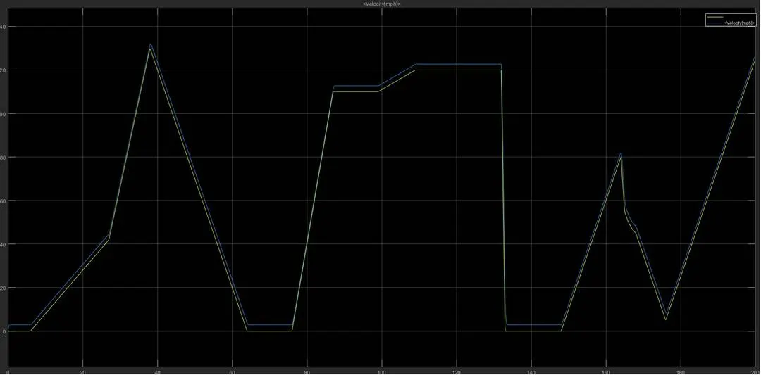
Finally, the output is taken as velocity in mph to plot the graph between time and velocity to obtain the drive cycle.

OUTPUT:-

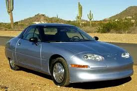
Solution4:- MODELING OF WOT(WIDE OPEN THROTTLE) OF GM EV1 CAR.

INTRODUCTION- The General Motor Produced The Ev1 Electric Car In 1996. It Was The First Mass- Produced And Purpose Designed Electric Car Of The Modern Era From a Major Automaker Company .and the first GM CAR designed to be electric.

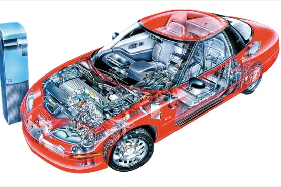
Car specifications

• Class=electric subcompact coupe
• Electric motor =102kw at 7000rpm and 149Nm at 0-7000 rpm
• Transmission -single-speed reduction integrated with motor and clutch
• Battery =18.7kwh(lead- acid) and 26.4kwh(nickel metal hydride)
• Range=89km(lead-acid)and 169km(nickel metal hydride)
• Wheelbase=2510mm
• Length=4310mm
• Width=1770mm
• Height=1280mm
• Kerb=1400kg(lead-acid)and 1319kg(nickel metal hydride)

WITH ORIGINAL PARAMETERS

• Drag Co-efficient (C_d) = 0.19
• Co-efficient of Rolling Resistance (= 0.0048
• Motor Speed (N) = 12000 rpm
• Frontal Area (A) = 1.8 m^2
• The efficiency of Drive Coupling (ƞ_g) = 0.95
• Gross Weight (m) = 1540 Kg
• Kerb Weight = 1400 Kg
• Pay Load = 140 Kg
• Gear Ratio (G) =11
• Tire Radius = 0.3 m
• Motor Torque (T_max) = 140 Nm
• Critical Velocity (v) = 19.8 m/s
• Critical Angular Speed (= 733 rad/s
• Constant Power = 102 KW
• The density of Air (ρρ) = 1.25 Kg/m^3
• Velocity for limiting acceleration (v) = 35.8 m/s

Calculations:-

Motor torque,`T=frac{F*r}{G}`

Tarctive force(`F_te`),

`F_te=frac{T*G}{R}

Total tractive force

`F_te=F_rr+F_ad+F_la+F_wa`

where:

• `F_rr`is the rolling resistance force
• `F_ad`is the aerodynamic drag
• `F_hc`is the hill-climbing force
• `F_la`is the force required to give linear acceleration
• `F_ωa`is the force required to give angular acceleration to the rotating motor

`frac{T⋅G}{r}=(μrr⋅m⋅g)+(0.5⋅ρ⋅A⋅Cd⋅v2)+(m)+(I⋅frac{G2}{r2⋅ƞg})⋅(frac{dv}{dt})`

In most cases at low speeds, the maximum torque is a constant until the motor speed reaches a critical value ωc">ωc (critical speed) after which the torque falls.

So, `T=T_max`

`frac{Tmax⋅G}{r}=(μrr⋅m⋅g)+(0.5⋅ρ⋅A⋅Cd⋅v2)+(m+I⋅(frac{G2}{r2⋅ƞg}))⋅(frac{dv}{dt})`

Here we donot have moment of inertia because as compare to the weight of the vehicle the moment of inertia is negligible so we consider 20kg moment of inertia.now m=1560kg

`(0.95*37*140)=72.4+(0.214*v^2)+1560*frac{(dv)}{(dt)}`

`Frac{dv}{dt}=3.11-0.000137*v^2---------------------------(A)

When the speed reached at v=19.8m/s,then the torque is

T=Tmax

`Tmax=frac{P}{v*37}`

`Tmax=frac{102000}{v*37}`

`Tmax=frac{2756}{v}`

`frac{0.95*37*2756}{v}=72.4+(0.214*v^2)+1560*frac{dv}{dt}

`frac{dv}{dt}=frac{62.1}{v}-0.046-0.000317*v^2--------------(B)

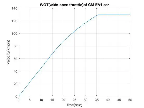
So, That motor limits the acceleration of the vehicle when the vehicle attains the speed of 35.8 m/s i.e., 128.86 Kmph. Till this speed the vehicle accelerates after that it runs at a constant speed so, no more acceleration is provided after 128.86 Kmph.

Equation A and B should be written in Finite Difference form,

`v_(n+1)=v_n+delt*(3.11-0.000137*(v_n)^2)`--------------(C)

`v_(n+1)=v_n+delt*((frac{62.1}{vn})–0.046–0.000317(v_n)^2)`------------(D)

Code:-

%WOT(wide open throtle)of GM EV1 car with orignal parameters
clear all 
close all 
clc
%electric scooter acceleration
t=linspace (0,50,201);  %0 top 50, in 0.1 sec steps 
vel=zeros(1,201); %501 readings  of velocity
d=zeros(1,201) %array for storing distance travelled 
dt =0.1; %0.1 second time step 

for n=1:200
   % now follow equations 
   if vel(n)<19.8 %  %torque constant till this point 
    vel(n+1)= vel(n)+dt*(3.11-(0.000137*(vel(n)^2)));
   elseif vel(n)>=35.8
       vel(n+1)=vel(n);
   else
    vel(n+1)=vel(n)+dt*(((62.1)/vel(n))-0.046-(0.000137*(vel(n)^2)));
   end 
end
vel = vel*3.6; % multiplying by 3.6 to m/s to km/h
M=max(vel)
plot(t,vel); 
axis([0 50 0 140])
title('WOT(wide open throttle)of GM EV1 car')
xlabel('time(sec)')
ylabel('velocity(kmph)')
grid on

       

PROCEDURE:-

• It creates a time array ‘t’ containing values from 0-50 sec.
• Then creating velocity ‘v’ vector with zeros to store the calculated values.
• Differentiation time ‘dt’ is checked for correct value.
• The looping statement starts
• Then the velocity ‘v’ is calculated till 19.8 m/s i.e.,71.28 Kmph from equation C.
• Then the compiler checks for the condition v>35.8 m/s i.e.,128.88 Kmph and if the condition fails it calculates the velocity from equation D.
• If the condition v>35.8 m/s i.e.,128.88 Kmph satisfies then it stops acceleration (calculating velocity) and it repeats the same velocity till the time value (constant speed).
• The looping statement ends.
• Then the velocity (m/s) is converted into Kmph.
• Then graph is plotted between time and velocity.

Output:-

CASE 2 – WITH 5% CHANGE IN ORIGINAL PARAMETERS

DATA FOR CALCULATIONS :-

• Drag Co-efficient (C_d) = 0.1995
• Co-efficient of Rolling Resistance (= 0.00504
• Motor Speed (N) = 12600 rpm
• Frontal Area (A) = 1.911 m^2
• Efficiency of Drive Coupling (ƞ_g) = 0.9975
• Gross Weight (m) = 1617 Kg
• Kerb Weight = 1470 Kg
• Pay Load = 147 Kg
• Gear Ratio (G) =11.55
• Tire Radius = 0.315 m
• Motor Torque (T_max) = 147 Nm
• Critical Velocity (v) = 20.49 m/s
• Critical Angular Speed (= 769.65 rad/s
• Constant Power = 107.1 KW
• Density of Air (ρρ) = 1.31 Kg/m^3
• Velocity for limiting acceleration (v) = 37.59 m/s

Calculation:-

Motor torque,` T=frac{F*r}{G}`

Tractive force(`F_te`),

`F_te=frac{T*G}{R}

Total tractive force

`F_te=F_rr+F_ad+F_la+F_wa`

where:

• `F_rr`is the rolling resistance force
• `F_ad`is the aerodynamic drag
• `F_hc`is the hill-climbing force
• `F_la`is the force required to give linear acceleration
• `F_ωa`is the force required to give angular acceleration to the rotating motor

`frac{T⋅G}{r}=(μrr⋅m⋅g)+(0.5⋅ρ⋅A⋅Cd⋅v2)+(m)+(I⋅frac{G2}{r2⋅ƞg})⋅(frac{dv}{dt})`

In most cases at low speeds, the maximum torque is a constant until the motor speed reaches a critical value ωc (critical speed) after which the torque falls.

So, `T=T_max`

`frac{Tmax⋅G}{r}=(μrr⋅m⋅g)+(0.5⋅ρ⋅A⋅Cd⋅v2)+(m+I⋅(frac{G2}{r2⋅ƞg}))⋅(frac{dv}{dt})`

Here we donot have moment of inertia because as compare to the weight of the vehicle the moment of inertia is negligible so we consider 20kg moment of inertia.now m=1637kg

`(0.95*37*140)=72.4+(0.214*v^2)+1560*frac{(dv)}{(dt)}`

`Frac{dv}{dt}=3.23-0.000152*v^2---------------------------(A)

When the speed reached at v=20.49m/s,then the torque is

T=Tmax

`Tmax=frac{P}{v*37}`

`Tmax=frac{107100}{v*37}`

`Tmax=frac{2894.59}{v}`

`frac{0.95*37*2894.59}{v}=79.94+(0.249*v^2)+1637*frac{dv}{dt}

`frac{dv}{dt}=frac{64.77}{v}-0.048-0.000512*v^2--------------(B)

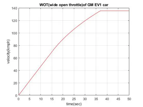
So, That motor limits the acceleration of the vehicle when the vehicle attains the speed of 37.59 m/s i.e., 1135.32 Kmph. Till this speed the vehicle accelerates after that it runs at a constant speed so, no more acceleration is provided after 135.32 Kmph.

Equation A and B should be written in Finite Difference form,

`v_(n+1)=v_n+delt*(3.23-0.000152*(v_n)^2)`--------------(C)

`v_(n+1)=v_n+delt*((frac{64.77}{vn})–0.048–0.000152(v_n)^2)`------------(D)

Code:-

%WOT(wide open throtle)of GM EV1 car with %5 change in parameters 
clear all 
close all 
clc
%electric scooter acceleration
t=linspace (0,50,201);  %0 top 50, in 0.1 sec steps 
vel=zeros(1,201); %501 readings  of velocity
d=zeros(1,201) %array for storing distance travelled 
dt =0.1; %0.1 second time step 

for n=1:200
   % now follow equations 
   if vel(n)<20.49 %  %torque constant till this point 
    vel(n+1)= vel(n)+dt*(3.23-(0.000152*(vel(n)^2)));
   elseif vel(n)>=37.59
       vel(n+1)=vel(n);
   else
    vel(n+1)=vel(n)+dt*(((64.77)/vel(n))-0.048-(0.000152*(vel(n)^2)));
   end 
end

vel = vel*3.6; % multiplying by 3.6 to m/s to km/h
M=max(vel)
plot(t,vel,'color','r'); 
axis([0 50 0 140])
title('WOT(wide open throttle)of GM EV1 car')
xlabel('time(sec)')
ylabel('velocity(kmph)')
grid on
       

PROCEDURE:-

• It creates a time array ‘t’ containing values from 0-50 sec.
• Then creating velocity ‘v’ vector with zeros to store the calculated values.
• Differentiation time ‘dt’ is checked for the correct value.
• The looping statement starts
• Then the velocity ‘v’ is calculated till 49m/s i.e.,73.76 Kmph from equation C.
• Then the compiler checks for the condition v>6m/s i.e.,135.3 Kmph, and if the condition fails it calculates the velocity from equation D.
• If the condition v>36m/s i.e.,135.3Kmph satisfies then it stops acceleration (calculating velocity) and it repeats the same velocity till the time value (constant speed).
• The looping statement ends.
• Then the velocity (m/s) is converted into Kmph.
• Then graph is plotted between time and velocity.

Output:-

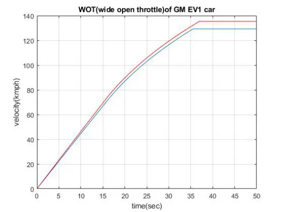
Comparing of plots:-

Now we comparing the original parameters with the 5%change parameters by combining both codes in a single one.

Code:-

%combining both data with orignal paremeters and 5% change in parameters 
clear all 
close all 
clc
%electric scooter acceleration
t=linspace (0,50,201);  %0 top 50, in 0.1 sec steps 
vel=zeros(1,201); %501 readings  of velocity
d=zeros(1,201) %array for storing distance travelled 
dt =0.1; %0.1 second time step 

for n=1:200
   % now follow equations 
   if vel(n)<19.8 %  %torque constant till this point 
    vel(n+1)= vel(n)+dt*(3.11-(0.000137*(vel(n)^2)));
   elseif vel(n)>=35.8
       vel(n+1)=vel(n);
   else
    vel(n+1)=vel(n)+dt*(((62.1)/vel(n))-0.046-(0.000137*(vel(n)^2)));
   end 
end
vel = vel*3.6; % multiplying by 3.6 to m/s to km/h
M=max(vel)
plot(t,vel); 
axis([0 50 0 140])
xlabel('time(sec)')
ylabel('velocity(kmph)')
grid on
hold on
for n=1:200
   % now follow equations 
   if vel(n)<20.49 %  %torque constant till this point 
    vel(n+1)= vel(n)+dt*(3.23-(0.000152*(vel(n)^2)));
   elseif vel(n)>=37.59
       vel(n+1)=vel(n);
   else
    vel(n+1)=vel(n)+dt*(((64.77)/vel(n))-0.048-(0.000152*(vel(n)^2)));
   end 
end

vel = vel*3.6; % multiplying by 3.6 to m/s to km/h
M=max(vel)
plot(t,vel,'color','r'); 
axis([0 50 0 140])
title('WOT(wide open throttle)of GM EV1 car')
xlabel('time(sec)')
ylabel('velocity(kmph)')
grid on

Output:-

CONCLUSION:-

We can verify the plots with the motor limit where there is no acceleration (constant speed) beyond,

Original Parameters (BLUE) =128.88 Kmph

5% change Parameters (RED) =135.32 Kmph