Derive Transfer Function of Suspension System of a Car

AIM: Derive transfer function of suspension system of a car and convert it into state space format with the help of MATLAB.

OBJECTIVES:

1. How hybrid electric cars can be operated more efficiently by autonomous driving systems?
2. a.) Derive the transfer function of the suspension system shown below.

Note- Mass m1 corresponds to a quarter of the total vehicle mass (minus the wheels), mass m2 corresponds to wheel. k1 and k2 are spring constants. c1 is the damper coefficient. u is the road surface displacement and z1 and z2 measures the position of the mass m1 and m2.

b.) Convert the transfer function to state space format.

c.) Perform the same in MATLAB using suitable commands.

3. Derive the transfer functions for the RC(output across C) and CR (output across R) circuits shown below. Are they equal?

Note: RC circuit: Vs= Input voltage, Vc= output voltage.

CR circuit: Vin=Input voltage, Vout= output voltage.

Introduction

Transfer Function

Transfer function will allow separation of the input, system, and output into three separate and distinct parts, unlike the differential equation. Transfer function will also allow us to algebraically combine mathematical representations of subsystems to yield a total system representation.

The transfer function of a linear, time-invariant, differential equation system is defined as the ratio of the Laplace transform of the output (response function) to the Laplace transform of the input (driving function) under the assumption that all initial conditions are zero.

Limitation of Transfer function analysis

Transfer Function: For any Linear Time Invariant system Laplace of Output Divided by Laplace of Input at Zero initial condition is called transfer function of system.

• Transfer Function is defined under Zero initial conditions.
• Transfer function approach can be applied only to linear time invariant systems.
• It does not give any idea about the internal state of the System.
• It can be only applied to SISO (Single input Single output) systems.
• It is comparatively difficult to perform transfer function analysis on computers.

What are State-Space Models?

• State Space control is often referred to as a “Modern” control method because it takes the differential equation that describes the Time Domain of the System and analyses them in vector form using state variables.
• This is in contrast to “Classical” Control methods, such as Transfer function, which rely on complex Laplace transforms.

What is State?

• The state of a system is the minimum set of variables (state variables) whose knowledge at time t = 0, along with the knowledge of the inputs at time t >= t0 completely describe the behavior of a dynamic system for a time t > t0.
• State variable is set of variables which fully describe a Dynamic system at a given instant of time.
• The number of the state variables required is equal to the number of the storage elements present in the system.
• The number of the state variables required is equal to double of the number of displacements in the Mechanical system.

Advantage of State variable analysis.

• It can be applied to non linear system.
• It can be applied to Time invariant systems.
• It can be applied to MIMO (Multiple input Multiple output) systems.
• It’s give idea about the internal state of the system.
• This makes it possible to evaluate the system via simple matrix algebra, which also allows multiple-input, multiple-output systems to be evaluated
• State space analysis is an excellent method for the Design and analysis of control systems.

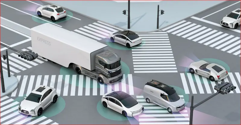
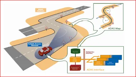
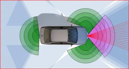
1.How hybrid electric cars can be operated more efficiently by autonomous driving systems? Abstract: Sensors are the eyes and ears of an automated vehicle. An automated vehicle has to detect other road users and should be able to interact with them in a safe way, hence it is important to understand what the vehicle's sensors should be capable of. We have investigated the different driving scenarios one can encounter in highway and rural environments, and sensing requirements have been derived for each of these scenarios. We have also listed the capabilities and drawbacks of different sensors, and have discussed possible solutions to enhance sensing performance and robustness. This thesis provides a good starting point for the selection of a sensor set for an automated vehicle. Autonomous Driving System

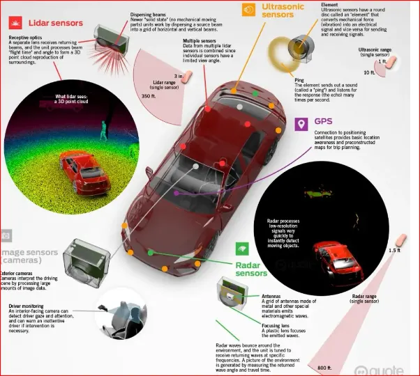
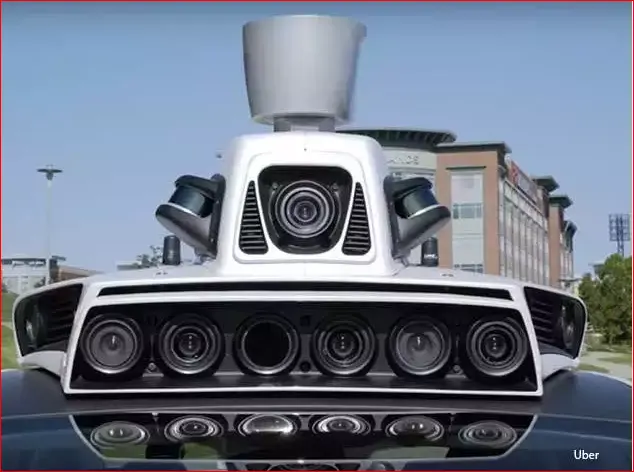
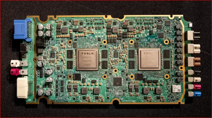
hybrid vehicles are the future of the modern automobile industries and making them autonomous is taking this vehicle to a different level making them autonomous is really difficult task and is also an expensive method for making them autonomous we required a lot of devices and those are - GPS - LIDAR - RADAR - Video Cameras - Central Computers Let us first discuss the first autonomous component GPS which stands for Global Positioning System. The GPS receiver calculates its own position and time based on data received from multiple GPS Satellite. Each satellite carries an accurate record of its position and time and transmits that data to the receiver. The GPS satellites carry very stable atomic clocks that are synchronized with other satellites and with ground clocks. Any drift from time maintained on the ground is corrected daily. In the same manner, the satellite locations are known with great precision. GPS receivers have clocks as well, but they are less stable and less precise. Let us now discuss the LIDAR which stands for Light Detection And Ranging this device is bulky devices compare to the other autonomous devices. Hybrid Vehicles may use LiDAR for obstacle detection and avoidance to navigate safely through environments. Point cloud output from the lidar sensor provides the necessary data for robot software to determine where potential obstacles exist in the environment and where the robot is concerning those potential obstacles. Singapore's Singapore-MIT Alliance for Research and Technology (SMART) is actively developing technologies for autonomous lidar vehicles. Lidar simulation models are also provided in autonomous car simulators. Now comes the RADAR in the autonomous Devices Which stands for Radio Detection And Ranging RADAR has been used in automotive for decades and can determine the velocity, range and angle of objects. It is computationally lighter than other sensor technologies and can work in almost all environmental conditions. Long-Range Radar (LRR) is the defacto sensor used in Adaptive Cruise Control (ACC) and highway Automatic Emergency Braking Systems (AEBS). Currently deployed systems have limitations and do not react correctly to certain conditions, such as a car cutting in front of your vehicle, detecting thin profile vehicles such as motorcycles being staggered in a lane and set distance based on the wrong vehicle due to the curvature of the road. To overcome the limitations. a radar sensor could be paired with a camera sensor in the vehicle to provide additional context to the detection and to avoid the error which is present in this autonomous device Video Cameras are also part of the autonomous devices as modern vehicles use them for better sign identification this all camera is powerful and also know the traffic signals and if the person is moving in ar any vehicle is moving or not. The camera sensor technology and resolution play a very large role in the capabilities. Cameras, similar to the human eye, are susceptible to adverse weather conditions and variations in lighting. But cameras are the only sensor technology that can capture texture, colour and contrast information and the high level of detail captured by cameras allow them to be the leading technology for classification. These features, combined with the ever-increasing pixel resolution and the low-price point, make camera sensors indispensable and volume leader for ADAS and Autonomous systems. The Central computers are the brain of the Autonomous System and these are the devices that control all devices and take control over the vehicle and records everything in the network of the vehicles. it takes the autopilot under the supervision of the driver. it takes care of all the ignition system in the vehicles and when autopilot is enabled your car to steer, accelerate and brake automatically within its lane. Current Autopilot features require active driver supervision and do not make the vehicle autonomous. Navigate on Autopilot suggests lane changes to optimize your route, and makes adjustments so you don’t get stuck behind slow cars

2.a.) Derive the transfer function of the suspension system shown below.

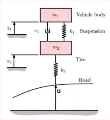
Note- Mass m1 corresponds to a quarter of the total vehicle mass (minus the wheels), mass m2 corresponds to wheel. k1 and k2 are spring constants. c1 is the damper coefficient. u is the road surface displacement and z1 and z2 measures the position of the mass m1 and m2.

Derivation of transfer function of a suspension system and converting it into a state space format

In the control design process the first step is to create a mathematical model of the system to be controlled. One of the ways to achieve this is by using the transfer function or the state space representation. The transfer function of a control system can be defined as the ratio of the laplace transform of the output variable to the laplace transform of the input variable with zero initial conditions. State space is a mathematical model of input, output and state variables related by first order differential equations or difference equations. Here we will see how to convert the transfer function into state space representation. Before that let us analyze the force balance equations of the idealized elements in the mechanical translational system.

• Mass Element.

Let us take an ideal mass element which has negligible friction and elasticity. Let F(t) be the applied force and F be the opposing force which is proportional to the acceleration of the body.

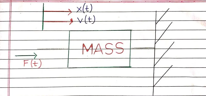
Here, let x be the displacement of mass and v is the velocity. The force can be calculated as -

`F=M dv/dt`

`=M (d^2 x)/(dt^2 )`

• Spring Element.

Let us consider an ideal elastic spring having negligible mass and friction. When a force is applied to it the spring offers an opposing force proportional to the displacement of the body.

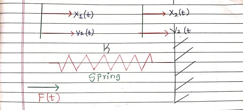
spring constant is k and when the spring has displacement at both ends then the force is proportional to differential displacement.

`F=k(x1-x2)`

`=kx`

`=k∫_(-∞)^t(v1-v2) dt`

`=k∫_(-∞)^tvdt`

• Damper Element.

Let us consider an ideal frictional element, damper which has negligible mass and elasticity and the diagram for the same is shown below. Let a force F(t) be applied to it. The dashpot offers an opposing force(F) proportional to the velocity of the body.

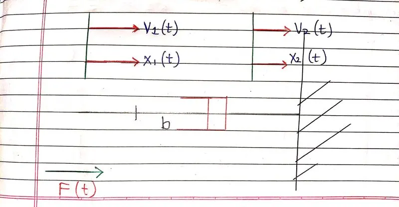
Here, the dashpot has displacement at both ends so the opposing force is proportional to the differential velocity. The damper coefficient is b and the force can be calculated as-

`F=b ( v1-v2)`

`=b (v)`

`=b((x1) ̇- (x2) ̇)`

`=bx ̇`

The state space representation of a system replaces an nth order differential equation with a single first order matrix differential equation. The state space representation of a system is given by two equations, the first equation is the state equation and the second equation is the output equation:

`q ̇(t)= Aq(t)+ Bu(t)`

`y(t)=Cq(t)+ Du(t)`

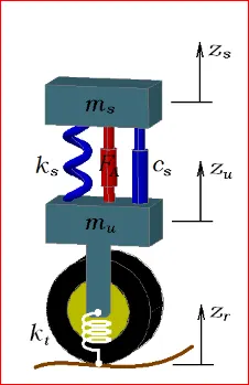
A quarter car model of a vehicle suspension is shown in the figure below. The model consists of a mass m1 corresponding to a quarter of the total vehicle mass (minus the wheels) and a mass m2 corresponding to a wheel. The suspension linking the vehicle body to the wheel consists of a spring of stiffness k1 in parallel with a shock absorber of damping coefficient c1. Meanwhile, the wheel is modeled as having a stiffness k2. Coordinates z1 and z2 measure the positions of masses m1 and m2 with respect to their static equilibrium positions (i.e., where the springs balance the gravity forces). The input to the suspension is the road surface displacement u, which is dependent on the road profile and vehicle speed.

First we will find the differential equations of both the masses. First we have to draw the free body diagrams of both the masses and then mark all the forces acting on the mass. The opposing force acts in a direction opposite to the applied force. The mass has to move in the direction of the applied force. Hence, the displacement, velocity and acceleration will be in the direction of the applied force. If there is no applied force then the acceleration, displacement and velocity of the mass will be in a direction opposite to that of opposing force.

The free body diagram for mass 1 is shown below. Also the differential equation is formed. Total force is equal to the sum of the forces applied by the spring and damper and mass.

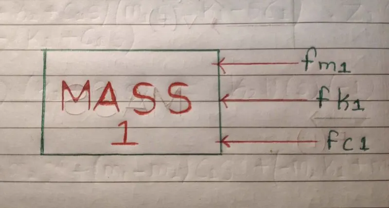
The forces are calculated as shown below. Force acting on mass is equal to the sum of the force of spring and damper and the mass itself.

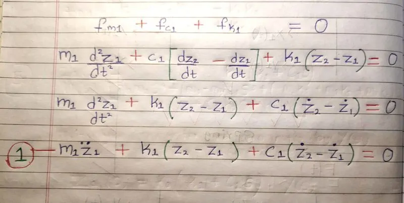
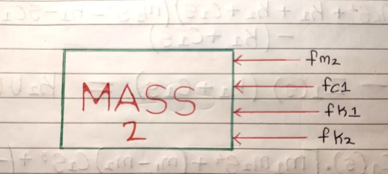
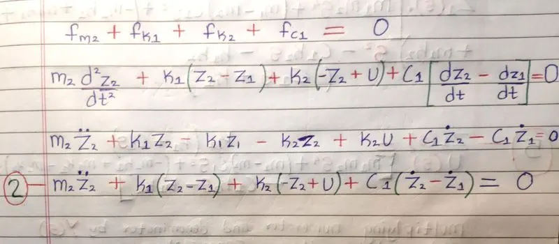
The free body diagram for mass 2 is shown below and the differential equation for this particular mass is noted. Total force on mass 2 is equal to the sum of the forces of both the springs and the damper and the mass.

Now we have to take the Laplace transform of differential equations to convert them to algebraic equations. After this the s-domain equations have to be rearranged to eliminate the unwanted variables and obtain the transfer function. The transfer function is to be converted into state space representation. For mass 1 we will form the transfer function from the differential equation. Laplace transform is taken for the equation. So, from equation (1) we can write as-

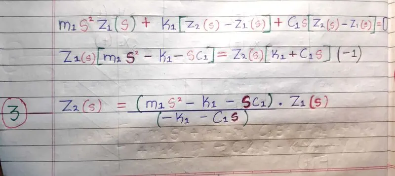
For mass 2 we have to form the transfer function. So, the Laplace transform is taken for the differential equation of mass 2. From equation (2) we can write as-

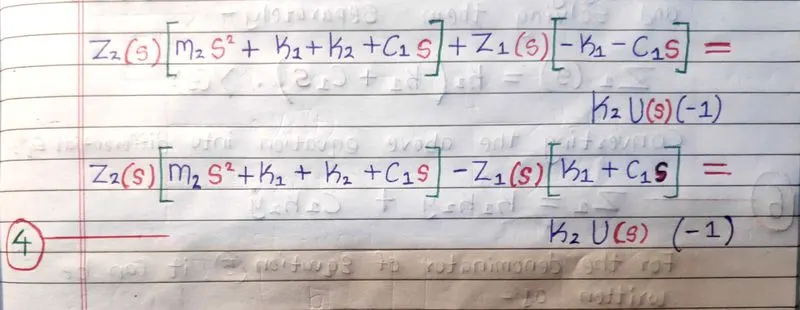
Putting the value of Z2 from equation (3) in equation (4). Now, the equation can be written as-

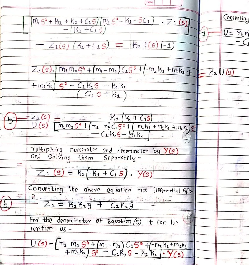
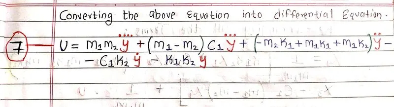
2.b.) Convert the transfer function to state space format.

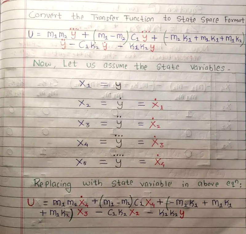
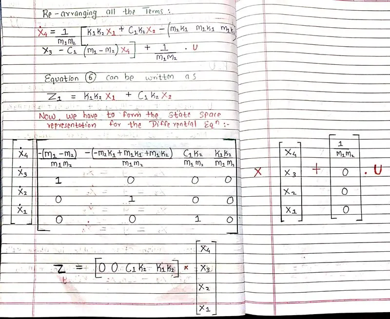
2.c.) Perform the same in MATLAB using suitable commands.

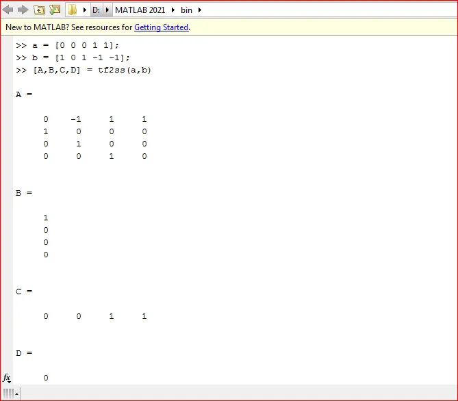
Thus, the transfer function for the suspension system is created and it is converted to its respective state space representation.

STEPS:

• expand the command prompt.
• type the required transfer function.
• change the transfer function to the state-space model by typing the command "tf2ss".
• press the enter.
• check for the error.

3. Derive the transfer functions for the RC(output across C) and CR (output across R) circuits shown below. Are they equal?

Note: RC circuit: Vs= Input voltage, Vc= output voltage.

CR circuit: Vin=Input voltage, Vout= output voltage.

Solution:

The transfer function of RC and CR circuits are not same because the output of RC circuit is across capacitor whereas the output for the CR circuit is across Resistor.

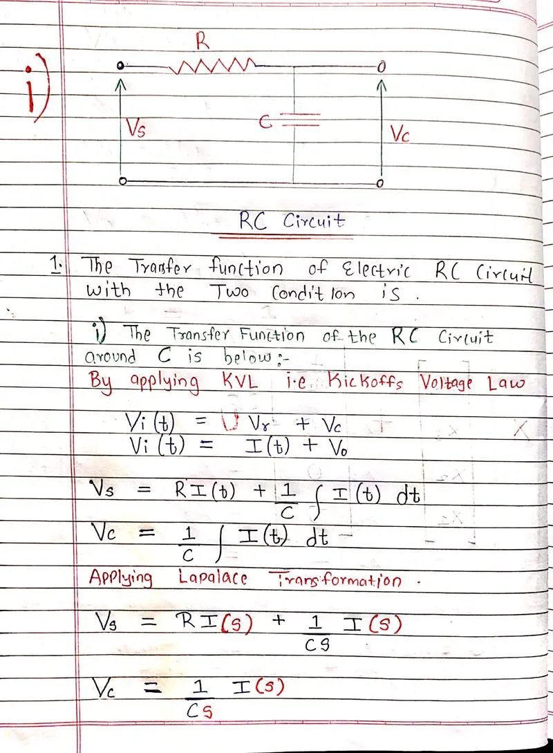
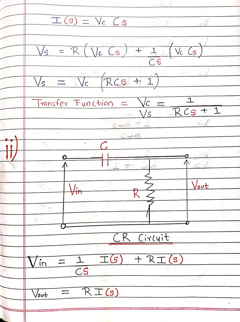
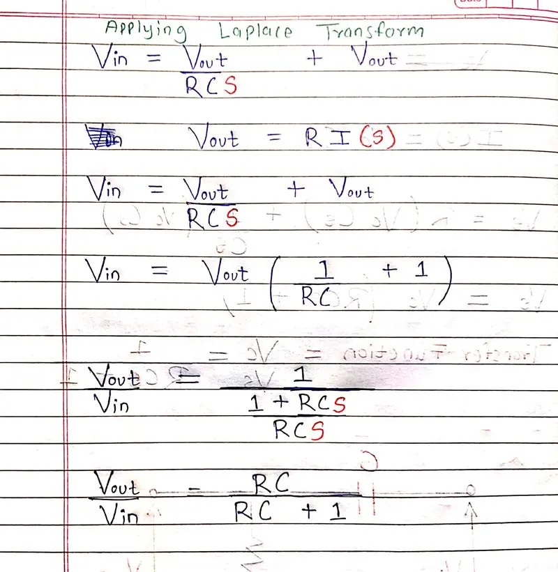
Hence, they are not equal. Changing the position of the capacitor and resistor in the circuit doesn't make a difference to the input voltage but it changes the output voltage, which is why the transfer function cannot be the same.

NOTES: https://drive.google.com/drive/folders/1txfFwkrjLX2JvtYvMHkxjd8AlDsG1eLB?usp=sharing

Conclusion:-

1. We all know that there are few disadvantages of autonomous vehicles due to the bulkiness of the devices used in that but in the coming time we will overcome that much
2. We got to find the method to convert the physical model of the spring, mass, damper and then converting into the transfer function, then converting into the state-space model.
3. From above we have concluded that both the transfer functions are different in both the terms in accordance to the C and R.

REFERENCE :

1. https://www.youtube.com/playlist?list=PLQ_iFGi3p1vJm8EZIZ6E9xr8MSeNXJaYD

2.https://www3.nd.edu/~pantsakl/Publications/348A-EEHandbook05.pdf

3.https://www.synopsys.com/automotive/what-is-autonomous-car.html