MATLAB Coding for working of Otto Cycle & to Calculate its thermal efficiency
Aim : To demonstrate the working of an Otto cycle and write a Matlab code to plot graph of PV diagram & calculate its thermal efficiency
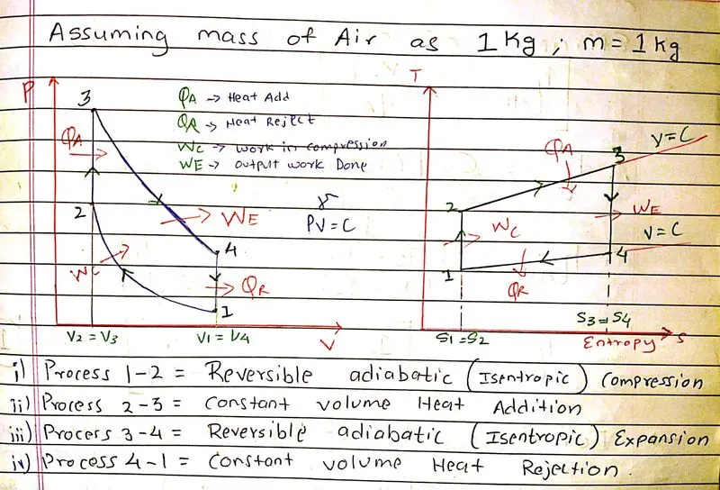
Theory : Air standard cycle ( Otto cycle): an Otto cycle is an idealized thermodynamic cycle that describe the function of a typical spark plug engine (petrol engine).It is most found in auto mobile engines.
- Process 1- 2 = Reversible adiabatic (Isentropic) compression.
- Process 2-3 = Constanmt Volume Heat Addition
- Process 3-4 = Reversible Adiabatic (Isentropic) Expansion.
- Process 4-1 = Constant Volume Heat Rejaction.
- Heat Addition at Constant Volume is given by :-
`Q_(A =) C_(v ) (T_3-T_2)` KJ/KG % mass = 1kg assume
- Heat rejection at constant Volume is given by
`Q_(R = ) C_v (T_4-T_1)` KJ/KG
- Work Done by Engine.
`W_D = Q_A- Q_R`
`W_D = C_v [(T_3-T_2 )-(T_4-T_1 )]`
- Efficiency of Otto cycle is given by :-
- `n_(Otto =) (W_D)/Q_A`
`n_(Otto =) 1- (T_4-T_1)/(T_3-T_2 )` equation no. 1
- For process 1-2 :-
`T_2/T_1 =(V_1/V_2 )^(γ-1)= (P_2/P_1 )^((γ-1)/γ)`
`r_c=compression ratio`
`r_c= V_1/V_2 =(cylinder volume )/(clearance volume)`
Therfore, `T_2=T_1 (r_c )^(γ-1)` equation no. 2
( Reversible Isentropic process )
`P_1 〖V_1〗^γ= P_2 〖V_2〗^γ`
`〖V_1〗^γ/〖V_2〗^γ =P_2/P_1`
- For Process 3-4 :- Reversible adiabatic process Expansion
- `V_1=V_4 ; V_3=V_(2 ) ( from p.v daigram)`
- `T_3/T_4 =〖V_4〗^(γ-1)/V_3 =〖V_1〗^(γ-1)/V_2 ; r_e=Expansion ratio`
- `T_3=T_4 (r_e )^(γ-1) □(⇒┴3 ) Equation no.3`
`Let r_c= r_e= r`
Put `“T_2” & “T_3”` in equation no. 1
Therefore, `〖 n〗_Otto=1-1/r^(γ-1)`
Result if “ r ” compression ratio increases then efficiency of Otto cycle increases.
- Piston Kinematic Equation
- How it’s combustion changes as the function of Crank angle
bore = 0.1
Stroke = 0.1
Con_rod = 0.15
Cr = 12
v_swept = pi/4*bore^2*stroke;
v_clearance = v_swept/(cr-1);
a = stroke/2 | ratio of con_rod to crank pin radius
R = con_rod/a
Formula for How volume inside the combustion chamber is going to change derived from pure geometric reletion
`V/V_c =1+1/2 (c_r-1)[ R+1-cos〖∅-(R^2-sin∅^2 ) 1/2 〗 ]`
theta = 0
term 1 = 0.5*(`c_r-1`)
term 2 = R +1 – cosd(theta) |cosd because cos in degree
term 3 = [ R^2 – sind(theta)^2]^0.5
V = [1 + term1*(term2 –term3)]*Vc
Points to remember :-
- To check the code runs correctly when theta is set to 0 then volume must correspond to clearance volume which is basically TDC volume i.e
- We covert the above formula into function so it could be reuse for varying value of theta.
- Name of the function and the name of the file should be same .
function [V] = engine_kinematics( bore, stroke, con_rod, cr, start_crank, end_crank )

a = stroke/2
R = con_rod/a

v_s = pi/4*bore^2*stroke;
v_c = v_s/(cr-1);


theta = linspace(start_crank,end_crank,100);


term1 = 0.5*(cr-1)
term2 = R + 1 - cosd(theta);
term3 = (R^2 - sind(theta).^2).^0.5;

V = (1 + term1*(term2 - term3)).*v_c;

end
Using the above code we could plot the pv daigram but yet it will not follow the path which it should be,because matlab code is just joining the points of compression, combustion, expansion,exhaust.
where on otherside it should follow th actuall path by taking each stages in account,it could be achieved by determining the constant K.
- K = PV^gamma is constant along the isotropic process,Where pressure times volume over gamma is going to be constant.
- If we determine this constant then we can say that doing isotropic process “P” times V_compression^gamma
P_compression*V_compression^gamma =constant_c
P_compression = constant_c./v_compression^gamma
 t2 = p2*v2*t1/(p1*v1)

 constant_c = p1*v1^gamma;
 V_compression = engine_kinematics(bore, stroke, con_rod, cr, 180,0);
 P_compression = constant_c./V_compression.^gamma;
From the above code we can determine P_compression and plot it against V_compression to follow the desired path.
Similarly we could determine Expansion stage,and plot V_expansion against P_expansion.
  p3 = p2*t3/t2

  constant_c = p3*v3^gamma;
 V_expansion = engine_kinematics(bore, stroke, con_rod, cr, 180,0);
 P_expansion = constant_c./V_expansion.^gamma;
Final plot following desired paths after adding Title & Label is Coded below :-
 figure(1)
   grid on;
   grid minor;
   hold on
   plot(v1,p1,'color','r','linew',3)
   plot(V_compression,  P_compression,'linew',3)
   plot(v2,p2,'color','b','linew',3)
   plot([v2 v3],[p2 p3],'linew',3)
   plot(v3,p3,'color','g','linew',3)
   plot(V_expansion, P_expansion,'linew',3)
   plot(v4,p4,'color','y','linew',3)
   plot([v4 v1],[p4 p1],'linew',3)


   %Adding the Labels
   xlabel('Volume in m^3')
   ylabel('Pressure in Pa')


   %Adding the Title
   title ('PV daigram of an IC engine ');
   legend('Compression','Combustion','Expansion','Exhaust');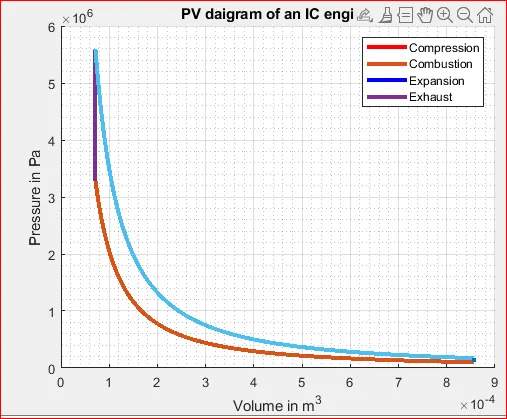
Output :- The thermal efficiency of the Cycle is given following code as mention below.
   %Calculating Thermal Efficiency
   thermal_efficiency = 1-1./cr^(gamma-1);

   %Print the thermal efficiency
   fprintf(['The thermal efficiency of the cycle is  : ' num2str(thermal_efficiency)]);
   fprintf('n');

Final Matlab Code :-
clear all
close all
clc
%Inputs
gamma = 1.4 ; t3 = 2300
%State variable at point 1
p1 = 101325
t1 = 500

%Engine gometric parameters
bore = 0.1;
stroke = 0.1;
con_rod = 0.15;
cr =  12;

%Calculating the swept volume and clearance volume
 v_swept = (pi/4)*bore.^2.*stroke;
 v_clearance = v_swept/(cr -1);
 v1 = v_swept +  v_clearance
 v2 = v_clearance

 %State vairable at state point 2
 %p2v2^gamma = p1v1^gamma
 %p2 = p1*(cr).^gamma
 p2 = p1*(cr).^gamma

 %Ideal Gas Law
 %p1v1/t1 = p2v2/t2
 %t2 = p2v2.*t1/(p1*v1)
 t2 = p2*v2*t1/(p1*v1)

 constant_c = p1*v1^gamma;
 V_compression = engine_kinematics(bore, stroke, con_rod, cr, 180,0);
 P_compression = constant_c./V_compression.^gamma;

 %State variable at state point 3
 v3 = v2

 %p3v3/t3 = p2v2/t2   | p3 = p2*t3/t2
  p3 = p2*t3/t2

  constant_c = p3*v3^gamma;
 V_expansion = engine_kinematics(bore, stroke, con_rod, cr, 180,0);
 P_expansion = constant_c./V_expansion.^gamma;


  %State variables at state point 4
  v4 = v1

  %p3v3^gamma = p4v4^gamma  | p4 = p3*(v3/v4)^gamma
   p4 = p3*(v3/v4)^gamma

   figure(1)
   grid on;
   grid minor;
   hold on
   plot(v1,p1,'color','r','linew',3)
   plot(V_compression,  P_compression,'linew',3)
   plot(v2,p2,'color','b','linew',3)
   plot([v2 v3],[p2 p3],'linew',3)
   plot(v3,p3,'color','g','linew',3)
   plot(V_expansion, P_expansion,'linew',3)
   plot(v4,p4,'color','y','linew',3)
   plot([v4 v1],[p4 p1],'linew',3)


   %Adding the Labels
   xlabel('Volume in m^3')
   ylabel('Pressure in Pa')


   %Adding the Title
   title ('PV daigram of an IC engine ');
   legend('Co   %Calculating Thermal Efficiency
   thermal_efficiency = 1-1./cr^(gamma-1);

   %Print the thermal efficiency
   fprintf(['The thermal efficiency of the cycle is  : ' num2str(thermal_efficiency)]);
   fprintf('n');

  mpression','Combustion','Expansion','Exhaust');
Conclusion :-
In this Report Otto cycle was studied and was plotted using Matlab,Important insights are obtained on the efficiency and the plotting of the cycle.Matlab is very powerful tool especially when it comes to numerical computing.
REFERENCE :