PART- I Wide Open Throttle (WOT) response of General Motors GM 1st EV Car
AIM :-
To Calculate Wide Open Throttle Condition (WOT) as per following Objectives and given parameter.
OJECTIVES :-
- Calculate the Ratio of hill – climbing power required by the fully loaded TATA Ultra Truck to the half loaded one.
- To calculate the minimum length of Flyover considering the minimum height of the Summit should be 5.5 meters.
- To prepare the new drive cycle excel file for the driver glider model and also include hill climbing angle to it.
- To model the WOT (Wide Open Throttle) response of GM Ev1 car & compare it with official figure of the performance of the real vehicle.
- To show the variation in acceleration time with a 5% change in vehicle parameters.
Introduction
Wide-Open Throttle –
WOT is also known as the highest acceleration peak when the motor operates at its full RMP to propel the vehicle. At this condition, the vehicle is at rest position and we apply full throttle with no time
For HEVs wide-open throttle depends upon traction, general motor, and engine to satisfy the driver demand for achieving its acceleration performance.
Different types of loads
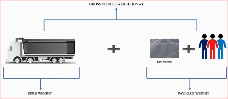
- Kerb weight (curb weight) :-
Kerb weight is one of the most important specifications of any vehicle. Kerb weight is the total mass of the vehicle with standard equipments and all required operating equipments such as Motor oil, coolant oil, transmission oil and from time to time fuel in the Fuel tank.
- PayLoad :-
Payload weight is defined as the number of goods or stuff a vehicle can carry safely.
- Gross Vehicle Weight :-
It is the maximum operating weight/mass of weight as specified by the manufacturer including vehicle’s chassis, body, engine, engine fluid ,fuel, accessories, driver, passengers and cargo but excluding that of any trailer.
- Gradeability of vehicle :-
Gradeability is define as the steepness of grade that a motor vehicle is capable of climbing at efficient speed or we can say that it is the highest grade a vehicle can ascend maintaining a particular speed.
Gradeability is measured in different ways,
- An angle of inclination to the horizontal.
- Percentage of rise over run.
- The ratio of one part runs to some particular number of parts.
Calculation :-
https://www.facebook.com/watch/?v=272053857739771
- What is the ratio of hill-climbing power ratio required by fully loaded TATA ultra-truck to the half-loaded one?
TATA Ultra 1012AC
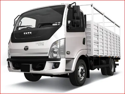
Technical specification
Engine type TATA 497 TCIC, water-cooled direct injection diesel
Engine Capacity (cc) 3783
Max Engine output 125 Ps at 2400 rpm
Max Engine Torque 400 Nm at 1300-1500 rpm
Wheel Base (mm) 3920
Overall Length (mm) 7139
Max width (mm) 2204
Kerb Weight (kg) 3120
GVW (kg) 10400
Gradeability 33%
Top Speed (kmph) 95
TATA Ultra 1012 AC
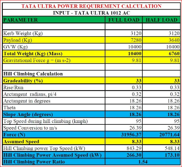
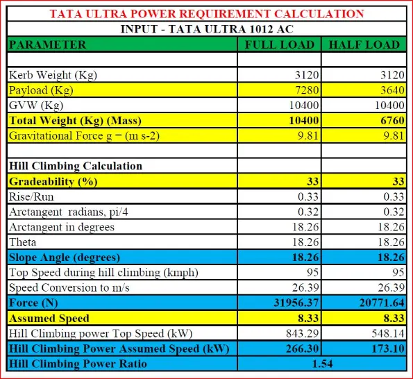
PARAMETER FULL LOAD HALF LOAD
Kerb Weight (kg) 3120 3120
Pay Load (kg) 7280 3640
GVW (kg) 10400 6760
Gravitational Force 9.81 9.81
Gradeability 33 33
Slope Angle (degree) 18.26 18.26
Top-Speed (kmph) 95 95
Assumed Speed (kmph) 30 30
FORMULA USED:-
- For calculating force
`F=M*g*sin(θ)`
M = mass
g = gravitational force
- Hill climbing force
`F_hc=M*g*sin(θ)` { for converting angle (degree) into radian `(π*θ)/180` }
- For Calculating power (kw)
`Power= (F*V)/1000`
- For Power ratio
`Power Ratio= (Full Load)/(Half Load)`
CALCULATION :-
Percent of slope (% Gradeability) to Degree
`tanθ= ((Rise)y( 5.5))/((Run)x (15.73))`
`θ= tan^(-1)〖y/x〗`
= 0.33
`θ=18.26°`
TATA Ultra 1012 Full Load Calculation
Kerb Weight = 3120
GVW = 10400
PayLoad = 10400 – 3120
= 7280 kg
Hill climbing force
`F=M*g*sinθ`
F = 10400 * 9.81* sin (3.14*18.26/180)
F = 31956.37 N
Calculation of Hill climbing power at top speed i.e. 95 kmph (26.39 m/s)
Power = (F *V)/1000
P = 843.29 kw
Calculation of hill climbing power at assumed Speed 30 kmph (8.33 m/s)
Power = (F *V)/1000
P = (31956.37*8.33)/1000
P = 266.30 Kw
Thus, TATA Ultra 1012 AC requires 31956.37 N Force and 266.30 Kw Power at full Load condition By Assuming Speed 30 kmph (8.33 m/s).
TATA Ultra 1012 Half Load Calculation
Kerb Weight = 3120
GVW = 10400
PayLoad = 10400 – 3120
= 7280 kg
Half PayLoad = 7280/2
= 3640 kg
Total weight = Half Payload + Kerb Weight
= 3640kg + 3120 kg
= 6760 kg
Hill climbing force
`F=M*g*sinθ`
F = 6760* 9.81* sin (3.14*18.26/180)
F = 20771.64 N
Calculation of Hill climbing power at top speed i.e. 95 kmph (26.39 m/s)
Power = (F *V)/1000
Power = (20771.64 *26.39)/1000
P = 5481.14 kw
Calculation of hill climbing power at assumed Speed 30 kmph (8.33 m/s)
Power = (F *V)/1000
P = (20771.64*8.33)/1000
P = 173.10 Kw
Thus, TATA Ultra 1012 AC requires 20771.64N Force and 173.10Kw Power at full Load condition By Assuming Speed 30 kmph (8.33 m/s).
Calculating Hill Climbing Power Ratio
`Power Ratio= (Full Load)/(Half Load)`
`Power Ratio= 266.30/173.10`
Power Ration = 1.54
Excel calculator Result for power Ratio
link :-https://drive.google.com/file/d/1rUvJxTTuMrYHFjQf2bZpIXoyE5tPzSVB/view?usp=sharing
2. https://www.facebook.com/watch/?v=272053857739771
- A flyover is planned to be constructed on National Highway. Keeping in mind about the Gradeability for truck , how much can be minimum length of flyover, considering the minimum height at the summit should be 5.5 meter ?
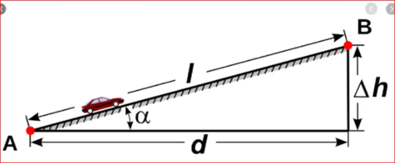
Data for calculation Flyover by using TATA Ultra 1012AC
Percent of slope (% Gradeability) to Degree
Percent of slope (% Gradeability) to Degree
`tanθ= ((Rise)y( 5.5))/((Run)x (15.73))`
`θ= tan^(-1)〖y/x〗`
= 0.33
`θ=18.26°`
For Calculating minimum length of Flyover.
Sin (theta) = (opposite side)/ Hypotenuse
0.33 = 5.5/ hyp
Hyp = 5.5/0.33
Hyp = 16.67 m
For Calculating minimum run of Flyover
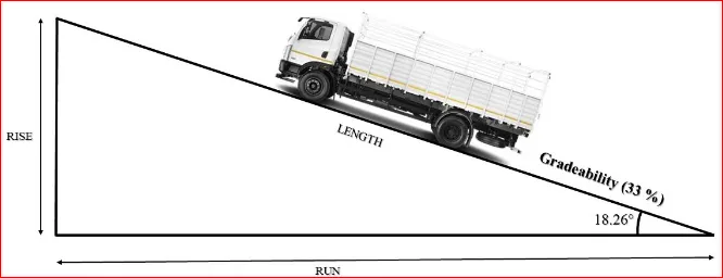
b = 15.73
For Calculating Total run of Flyover
= b * 2
= 15.73 * 2
= 31.46 m
Thus, the minimum length of the Flyover is 16.67 meters
Excel Calculator Result for the Flyover
3.Refer to the Below Link :
Prepare a new drive cycle excel file for the model above and also include a hill-climbing angel to it . Revise the model and comment on the results.
- First , we have to create a new drive cycle by using MS Excel and save with a proper name so that it will be easy call in MATLAB
- Open MTLAB and navigate The folder location set your working directory.
- After that, we have to import the Excel File in MATLAB by using “Import Data” command.
- Now a new window will open which shows the imported Excel Data, where we have to change the output type “Table to Numerical Matrix”
- The numerical matrix defines the type of MATLAB variable to import, now click on import.
- The new Drive Cycle will be imported and save in the Workspace.
- Now go to New and select Simulink Model and Open the Driver_Glider.slx file.
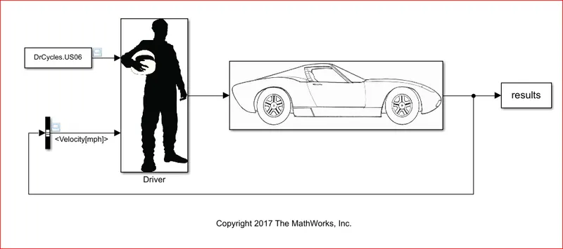
- Now we have to replace our Imported Excel Drive cycle with the Input of the Model Drive cycle of the above model.
- Drive Cycle Link :-https://drive.google.com/file/d/1dFNTibmF7FI3YOe6FIzQH1Rx2zAhkqL9/view?usp=sharing
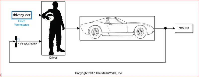
- Double click anywhere on window and type “From Workspace” and change name to your Excel file name which in our case is driverglider.

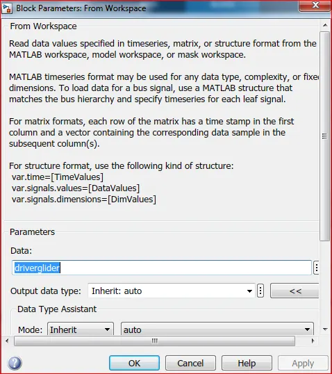
- Delete the DrCycle.US08 block and replace it with our from workspace block and Run the model.
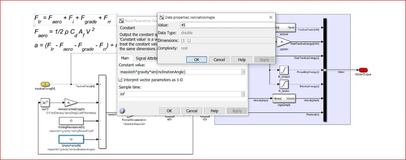
- Now for changing the grade force double click on the glider model, a new window will open where we can set inclination angel to find the grade force.
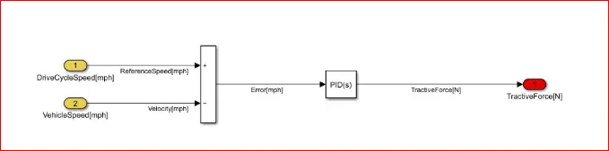
- This shows the PID controller for the Driver.
Output Result :-
Blueline Represents the fixed velocity whereas yellow line is changed in velocity due to change in inclination angle or Grade Force.
Result_1
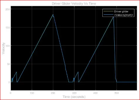
The above Graph shows the Velocity vs Time
Result_2
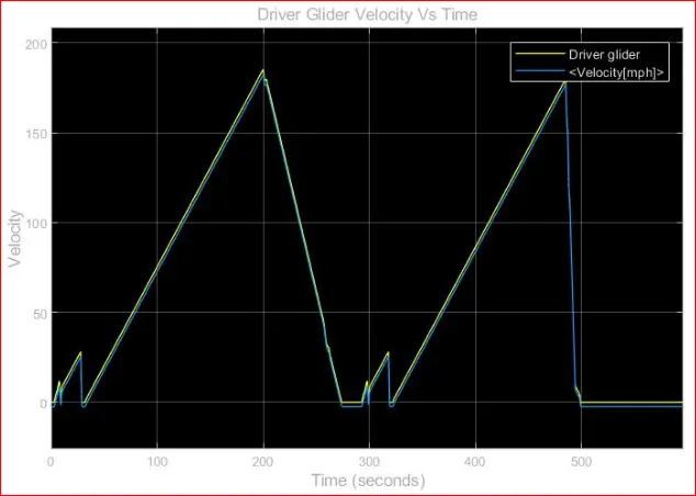
As we enter the inclination angle then we will see change in velocity.
4. Model the WOT (Wide Open Throttle) response of GM EV1 car. Compare it with the official figure for the performance of a real vehicle. Prepare a table showing variation in acceleration time with a 5% change in vehicle parameters.
GM EV1 Details
The General Motors EV1 was an electric car produced and leased by General Motors from 1990 to 1999. It was the first Mass-produced and purpose designed electric vehicle of the modern era from a major Automaker, the 1st GM car designed to be an electric vehicle from the outset along with being the first and only passenger car to be marketed under the corporate General Motor (GM) name instead of being branded under one of its divisions.
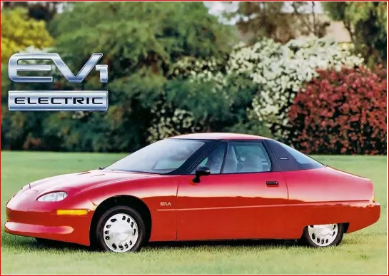
General Feature of GM EV1 car :-
- Aerodynamic Drag Coefficient (cd) = 0. 1 9
- Rolloing Resistance = 0.0048
- Induction Motor Max Speed = 12000 rmp
- Frontal Area (A) = 8 m^2
- Kerb Weight = 1400kg
- PayLoad = 160kg
- Total weight = 1560kg
- Critical velocity = 3kmph
- Gear ratio = 11:1 (G=11)
- Tyre Ratio = 30m
- Motor Max Torque = 140Nm
- Motor Speed = 733 rad
- Efficiency = 95 = 95%
By Using the Excel Calculator, We can easily find the 5% increase in vehicle parameters. The calculated value is shown in fig
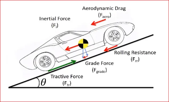
Formula Used :-
- Rolling Resistance `(F_rr )= μ_rr*Total weight(mg)`
- `μ_rr=Coefficient of rolling resistance`
- `Aerodynamic drag= 1/2*ρ*v^2*C_d`
- `Total power=(F_rr+F_ad )*Velocity/1000`
- `Hill Climbing Power=Total force* Velocity/1000`
- `Acceleration Force=Total Force- Hill Climbing Force-Tractive Force`
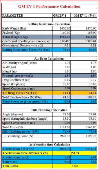
Solving by using simple differential equations.
Calculating the above critical Speed of motor i.e 102 kw
So,
`= G/(Tyer Radius)`
`= 11/0.3`
= 36.66 or 37v
Now
= 102*1000
=102000
We know
=`102000/(37*v)`
Now by using 2 equation
`G/r T=μ_rr*mg+0.625*A*C_d*v^2+(m+I G^2/(n_g r^2 )) dv/dt` ………………..Eq (1)
`F_te=μ_rr*mg+0.625*A*C_d*v^2+(ma+I G^2/(n_g r^2 ))a` …………….Eq (2)
Now we have two Equations
In the above Equations
G = Gear
T = Torque
r = Tyre radius
`μ_rr` = Rolling resistance
m = Mass of vehicle
g = gravitational force
A = Frontal area m^2
`C_d` = Aerodynamic Drag coefficient
V = Velocity
I = Moment of inertia
Motor equation
(Below critical speed)
(Above critical speed)
Solving the normal parameter of GM EV1 by using the above 2 equation.
Putting GM EV1 1 Parameter in Equation 1
= 11/0.3 * 0.95*140 = (0.0048 *1560*9.81) + (0.625*1.8* v^2*0.19) + (1560 *dv/dt)
= 366.66 * 0.95*140 = (0.0048 *1560*9.81) + (0.625*1.8* v^2*0.19) + (1638*dv/dt)
= 4875.78 = 73.45 + 0.213 v^2 + 1560 dv/dt
= 4802.33 = 0.213 v^2 + 1560dv/dt
dv / dt = 2.92 - 0.00013365v^2 ………………………. Eq (3)
Putting GM Ev1 Parameter in Equation 2
= 0.95* 36.66* 2757/v = 73.45 + 0.213 v^2 + (1560) dv/dt
= 96018/v = 73.45 + 0.213 v^2 + 1560 dv/dt
= dv/dt = 61.55/v – 0.047 – 0.0001365 v^2 …………………………….Eq (4)
MATLAB CODE :-
 clear all
 close all
 clc

 % Solving for normal parameter of GM EV1

 time1 = linspace(0,50,501);                 % 0.15 time step in seconds
 Velocity = zeros(1,501);                    % Velocity step count
 dv =  zeros(1,501);                          % Differentiate velocity
 dt  =  0.15 ;                               % change in time

 for n = 1:500
     % Calculation below critical speed
     if Velocity(n) < 19.8

         % By using Equation no.3 to evaluate constant Torque.
         Velocity(n+1) = Velocity(n) + dt*(3.07-0.0001365*Velocity(n)^2);

     elseif Velocity(n)<= 35.8    %Velocity reaches at top speed
         Velocity(n+1) = Velocity(n);

         % By using equation no. 4 to evaluate at typical power
     else
         Velocity(n+1) = Velocity(n)+ dt*(61.55-0.047*Velocity(n)-0.0001365*Velocity(n)^2);
     end
 end
 dv(n+1)  =  dv(n)+0.1*Velocity(n);    % Velocity data to match zero

 for  i  = 1:500
     if(Velocity(i)==Velocity(i+1))
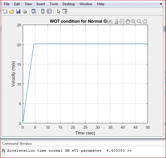
         fprintf('Acceleration time normal GM eV1 parameter  %f ',time1(i));
         break
     end
 end

 plot(time1,Velocity)
 hold on
 xlabel('Time (sec)')
 ylabel('Velocity (m/s)')
 grid on;
 title('WOT condition for Normal GM EV1 ')
Plotted Graph :-
Solving For 5% increase in the Parameter of GM EV1 by using the same above Equations.
Putting GM EV1 1 Parameter in Equation 1
= 11/0.3 * 0.95*140 = (0.00504*1638*9.81) + (0.625*1.8* v^2*0.19) + (1638 *dv/dt)
= 366.66 * 0.95*140 = (0.00504 *1638*9.81) + (0.625*1.8* v^2*0.19) + (1638 *dv/dt)
= 4875.78 = 80.98 + 0.213 v^2 + 1638 dv/dt
= 4794.8 = 0.213 v^2 + 1638 dv/dt
dv / dt = 2.92 - 0.0001300 v^2 ………………………. Eq (5)
Putting GM Ev1 Parameter in Equation 2
= 0.95* 36.66* 2757/v = 80.98 + 0.213 v^2 + (1638) dv/dt
= 96018/v = 80.98 + 0.213 v^2 + 1638 dv/dt
= dv/dt = 58.61/v – 0.049 – 0.0001300v^2 …………………………….Eq (6)
MATLAB CODE :-
 clear all
 close all
 clc

 % Solving for normal parameter of GM EV1

 time2 = linspace(0,50,501);                 % 0.15 time step in seconds
 Velocity2 = zeros(1,501);                    % Velocity step count
 dv =  zeros(1,501);                          % Differentiate velocity
 dt  =  0.15 ;                               % change in time

 for n = 1:500
     % Calculation below critical speed
     if Velocity2(n) < 19.8

         % By using Equation no.5 to evaluate constant Torque.
         Velocity2(n+1) = Velocity2(n) + dt*(2.92-0.0001300*Velocity2(n)^2);

     elseif Velocity2(n)<= 35.8    %Velocity reaches at top speed
         Velocity2(n+1) = Velocity2(n);

         % By using equation no. 6 to evaluate at typical power
     else
         Velocity2(n+1) = Velocity2(n)+ dt*(58.61-0.049*Velocity2(n)-0.0001300*Velocity2(n)^2);
     end
 end
 dv(n+1)  =  dv(n)+0.1*Velocity2(n);    % Velocity data to match zero

 for  i  = 1:500
     if(Velocity2(i)==Velocity2(i+1))
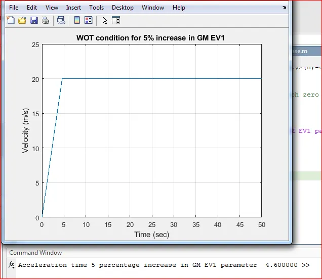
         fprintf('Acceleration time 5 percentage increase in GM EV1 parameter  %f ',time2(i));
         break
     end
 end

 plot(time2,Velocity2)
 hold on
 xlabel('Time (sec)')
 ylabel('Velocity (m/s)')
 grid on;
 title('WOT condition for 5% increase in GM EV1 ')
Plotted Graph :-
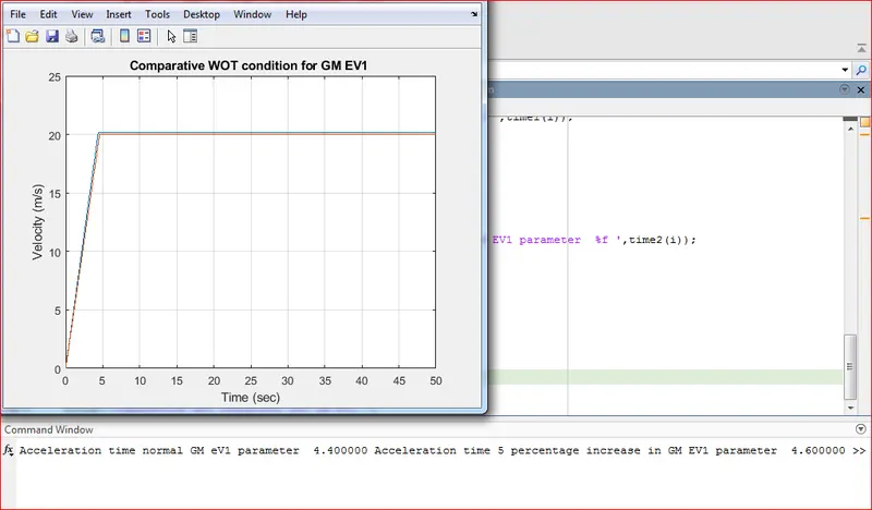
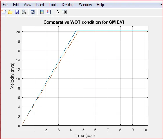
Now we will use Equation 3, 4, 5 and Equation 6 for Calculating the WOT Condition of GM EV1 by Using MATLAB scripting and plotting.
MATLAB CODE :-
 clear all
 close all
 clc

 % Solving for normal parameter of GM EV1

 time1 = linspace(0,50,501);                 % 0.15 time step in seconds
 Velocity = zeros(1,501);                    % Velocity step count
 dv =  zeros(1,501);                          % Differentiate velocity
 dt  =  0.15 ;                               % change in time

 for n = 1:500
     % Calculation below critical speed
     if Velocity(n) < 19.8

         % By using Equation no.3 to evaluate constant Torque.
         Velocity(n+1) = Velocity(n) + dt*(3.07-0.0001365*Velocity(n)^2);

     elseif Velocity(n)<= 35.8    %Velocity reaches at top speed
         Velocity(n+1) = Velocity(n);

         % By using equation no. 4 to evaluate at typical power
     else
         Velocity(n+1) = Velocity(n)+ dt*(61.55-0.047*Velocity(n)-0.0001365*Velocity(n)^2);
     end
 end
 dv(n+1)  =  dv(n)+0.1*Velocity(n);    % Velocity data to match zero

 % Solving for 5% increase in parameter of GM EV1
 % Solving for normal parameter of GM EV1

 time2 = linspace(0,50,501);                 % 0.15 time step in seconds
 Velocity2 = zeros(1,501);                    % Velocity step count
 dv =  zeros(1,501);                          % Differentiate velocity
 dt  =  0.15 ;                               % change in time

 for n = 1:500
     % Calculation below critical speed
     if Velocity2(n) < 19.8

         % By using Equation no.5 to evaluate constant Torque.
         Velocity2(n+1) = Velocity2(n) + dt*(2.92-0.0001300*Velocity2(n)^2);

     elseif Velocity2(n)<= 35.8    %Velocity reaches at top speed
         Velocity2(n+1) = Velocity2(n);

         % By using equation no. 6 to evaluate at typical power
     else
         Velocity2(n+1) = Velocity2(n)+ dt*(58.61-0.049*Velocity2(n)-0.0001300*Velocity2(n)^2);
     end
 end
 dv(n+1)  =  dv(n)+0.1*Velocity2(n);    % Velocity data to match zero

 % Normal GM EV1
  for  i  = 1:500
     if(Velocity(i)==Velocity(i+1))
         fprintf('Acceleration time normal GM eV1 parameter  %f ',time1(i));
         break
     end
  end

  % 5% increase in GM EV1
   for  i  = 1:500
     if(Velocity2(i)==Velocity2(i+1))
         fprintf('Acceleration time 5 percentage increase in GM EV1 parameter  %f ',time2(i));
         break
     end
   end

   %Plotting
    plot(time1,Velocity,time2,Velocity2)
 hold on
 xlabel('Time (sec)')
 ylabel('Velocity (m/s)')
 grid on;
 title('Comparative WOT condition for GM EV1 ')
Plotted Graph :-
CONCLUSION :-
- Thus from above we can say that increase in vehicle parameter leads in increase of Acceleration Time
- Minimum length of Flyover = 16.67 meters.
- Thus, Ratio of Hill Power for Fully and Hlaf Loaded is 1.54.
- the new Drive prepared in Excel and Replaced it with Driver glider model and Simulated using Hill Climbing angle as 45degree.
- the 5 % Change in Vehicle Parameter leads to increase Acceleration time.
REFFERENCE :-
https://drive.google.com/file/d/1YiDuswwR2Oj0kW6fYTqzqoImkp-SBzKr/view?usp=sharing