Week 6: Conjugate Heat Transfer Simulation

Conjugate heat transfer simulation:

Conjugate heat transfer happens when heat transfer happens between fluid to solid or vice versa and different mode of heat transfer like conduction and convection are involved in the process.

Creating geometry: Create cylinder from the ‘shapes ‘ option. This is having radius of 0.015m . Again draw a cylinder having radius of 0.002m with the same centre (origin).

Remove the faces of the cylinders from both sides and patch the edges again to form the thickness portion. Also patch the inlet and outlet flow faces. There will always be a non-manifold edge error visible in these conjugate heat transfer problems because the interface where different region lie on both side occur. Edges of many triangle meshes overlap with each other when non-manifold error occurs.

Velocity calculation by reylonds number:

Re=(ρ.V.D)/µ

Re=7000

ρ i.e density=1.184 at 300K

µ=1.840 x 10^(-5) m2/s at 300k

D=0.015mm

This gives velocity of 7.25m/s. This is taken as dirchilet BC for inlet condition.

After the diagnosis check for error and creation of boundaries, also check the normal direction. Case set-up is required as the next step:

Boundary conditions-

Inflow-

Boundary type-inflow, stationary boundary which is fixed , ‘law of wall’ applies here, velocity -7.25m/s

Region-Fluid region (stream ID 0)

Outflow-

Boundary type- outflow, stationary boundary which is fixed, ‘law of wall’ applies here.

Region-Fluid region(stream ID 0)

Solid outer wall –

Boundary type- wall, having heat flux of 10000W/m2 going into the system with ‘slip’ condition.

Region-Solid region(stream ID 1, solid)

The solid outer wall is made of aluminium and the fluid travelling inside is air.

Solid thickness- Boundary type- wall, ‘slip’ condition.

Region-Solid region(stream ID 1, solid)

Temperature boundary condition- Neumann, zero normal gradient

Interface-

The boundary separating them is named as interface. This consists of separate boundaries for the solid side and for the fluid side. The direction in which normal are pointing is the forward region . In our simulation , direction of normal is towards the fluid region. So, the forward region is fluid region and the reverse region is solid region. Boundary condition for fluid region will be given ‘law of wall’ and solid region will be given ‘slip’ condition for velocity and ‘specified value’ for temperature.

Base grid- 3 cases of base grid are taken here to compare the results. Mesh size 1-0.002mm , Mesh size 2- 0.004mm, Mesh size- 0.006mm.

Super cycling &its effects:

- The super cycling begins at 0.05 seconds. 0.01, 0.02,0.03 mm are the three cases considered for the length interval of the cycle. Interval of 0.01 means that when transient simulation will be carried out initially, supercycling will start at 0.05 secs . For the time when super cycling is performed, solid region simulation will be done by a steady solver and fluid region is freezed for that time. This is done in order to bring the solid and fluid region both at same temperature. Once, they are same then again for 0.01 sec transient simulation is ran, then again we stop and then again transient at 0.01 seconds. Solids have more capacitance, more specific heat, they take more time to achieve at a certain temperature whereas liquids &gases have lower specific heats, they change their temperatures fast i.e. they are more sensitive to temperature. This is why we need to pause the fluid part of simulation at some intervals and let the solid region also achieve that temperature. This is the time when transient simulation will be carried out. Super-cycling helps to fasten the process this way by performing the solid part of simulation (to equalise the temperature) with a help of a steady state solver. Different stage intervals are set and comparison for the temperature plots are shown in this report.

Observations &explanations:

Increase in cell count that occurred on post -processing for different mesh sizes:

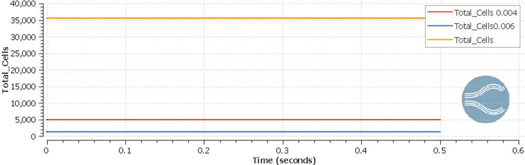
Cell count for mesh size of 0.006mm-2000 cells

Cell count for mesh size of 0.004mm-5000 cells

Cell count for mesh size of0.002mm-35000 cells

cells number increase as the cells become smaller in size

Plot for variation of temperature due to different mesh sizes, this shows grid dependence:

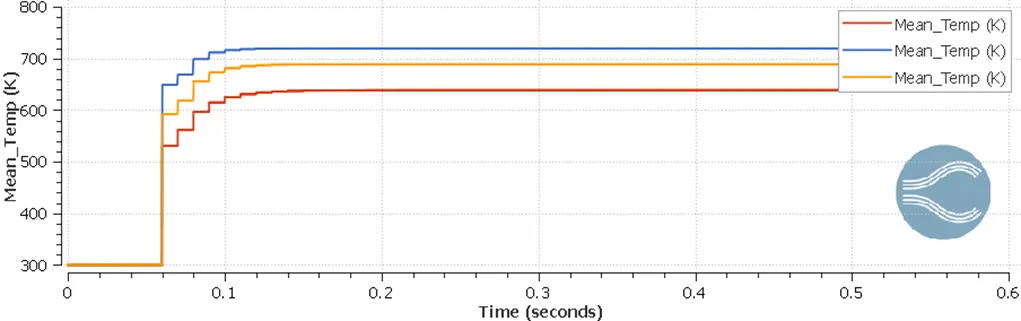
As per the ability for refining the results, with the current system specification, we can say that the grid is dependent. As we change the mesh size ,ideally there should not be any difference in plot images i.e. grid should be independent, but here we can see a slight difference in the temperature plots. As the mesh refines, i.e. becomes smaller in size , the mean final temperature becomes lower.

Plot for variation of temperature as per variation in Length of super cycling interval stage:

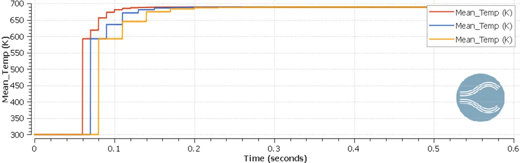
As the length interval for super cycling changes to 0.01 s, 0.02s,0.03s , then mean temperature plot reduces. We Increased the length of interval for which transient simulation runs and increasing this interval, the length of the step that the graph makes each time increases, i.e. for time interval increased. Ultimately, final temp will have no difference due to this time interval change, but it is just that we increased the amount of time for carrying out the simulation each time. The 0.03s interval converges the solution a little slower than the 0.01s interval because there simulation is carried out every 0.01 seconds and this helps solution converge earlier than if a longer interval is taken.

Red- length interval 0.01s

Blue- length interval-0.02s

Yellow -length interval-0.03s

Mesh size 0.002mm :

Mesh size 0.004mm :

Mesh size 0.006mm :

Variation of y plus image with mesh size:

Turbulent region is divided into a sub-laminar region and a turbulent region in which no viscous forces apply. Because the sub-laminar region, where viscous forces apply is too small. We need a smaller mesh size to simulate that region, whereas we can use bigger mesh size for turbulent region which occupies most area in the flow. The value of y plus tells us how coarse or fine the grid is. Y+ value <10 means sub-laminar region and y+ > 30 means turbulent region. Y+< 10 says that no slip condition will apply, we don’t need wall functions but y +>30 says that wall functions will be applied.

For size 0.002mm:

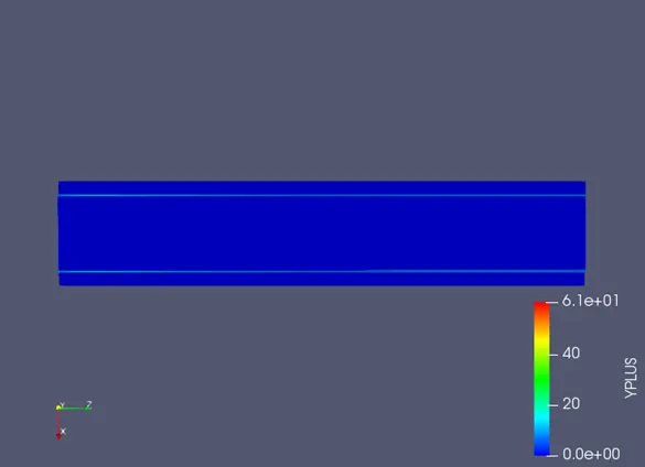
Wall functions will not be applied here as the y+ value is everywhere below 10.

For size 0.004 mm:

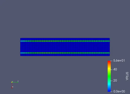
Y+ value everywhere except interface is in laminar region. At interface the value is in either in transition or turbulent region.

For size 0.006mm:

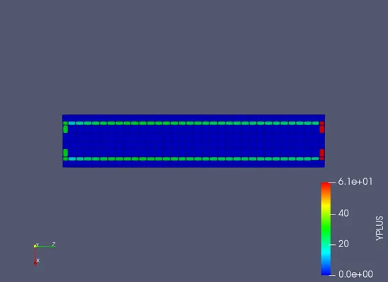
Y+value is mostly less than 10 in each region except interface, where y+ is in turbulent region i.e. greater than 30, specially at the outlet region of interface.

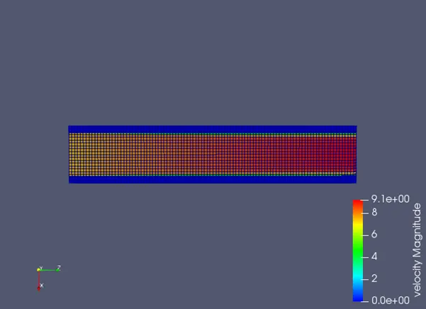
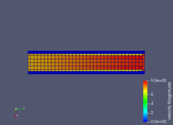
Velocity images for simulation:

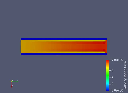
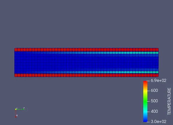
Temperature images for simulation:

Heat flux goes from the outer solid wall inside the cylinder towards the fluid region.

Mesh image 0.002mm:

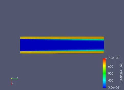
Mesh image 0.004mm:

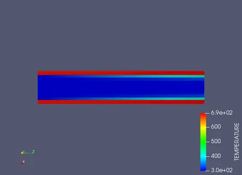
Mesh image 0.006mm:

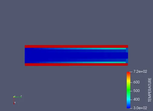
Video for temperature simulation:

Conclusion: Effects on temperature plots due to change in intervals of supercycling and on change of grid size in the flow of fluid in a cylindrical passage is seen where conjugate heat transfer is studied. The outer aluminium wall inputs a heat flux and the simulation plots agree with the theortical results. Also, super cycling helped the simulation to achieve results faster in the conjugate heat transfer scinaerio. Hence, the simulation perfomed is as per the theortical results.