Week 4 - CHT Analysis on Exhaust port

Q1.What is a CHT analysis and why is it used?

A conjugate heat transfer analysis is used when heat transfer i.e. conduction and convection are occurring. CHT analysis is used to solve the problem considering the heat transfer effects and hence can solve the heat transfer coefficients involved. In the given problem of exhaust port simulation, the exhaust from the 4 inlet pipes rushes to the outlet pipe of the exhaust. The exhaust is a high temperature at inlet and even increases its temperature after mixing at the outlet junction. The heat from the flue gases in the port transfer the heat through convection to the wall of the exhaust port solid body. Heat transfers by conduction from inner wall of the exhaust port wall to the outer wall , which transfers the heat to the ambient air in contact through convection.

Performing a CHT analysis can help find out the wall adjacent temperature, individual nodal heat transfer coefficients.

Therefore, when a thermal energy exchange at the interface of a solid and liquid domain happens, a CHT analysis is used.

Step used for running the simulation:

1-Import geometry for exhaust port. Repair duplicate edges first and then in prepare go to extract volume and select the edges at the opening for inlets and outlet. This creates a separate fluid volume.

Very important: Share topology always, combine both volumes in one component and delete empty components. Go to workbench and click on share prep always after these steps. This creates a conformal mesh which is required for conjugate heat transfer analysis.

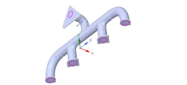
2-Go to meshing. Create named selection-inlet, outlet, Outerwall convection and inflation layer named selection. Mesh size-150mm, Quality> check the ‘Element quality’ option.

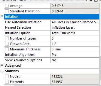
Inflation>all faces in chosen named selection> named selection of inflation layers (this is done by hiding the upper face and selecting the interface, this is basically the internal fluid volume that was created in space claim in first step.)

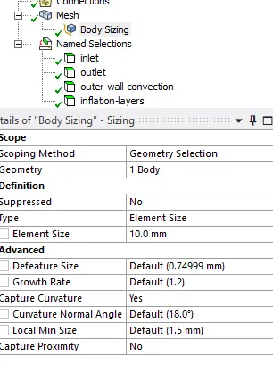
Now insert sizing to create a 10mm mesh specifically for the solid volume .It is very important to capture curvature> yes.

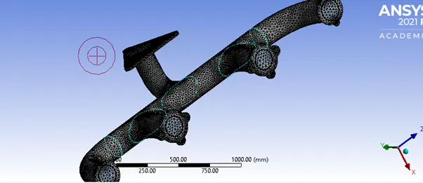
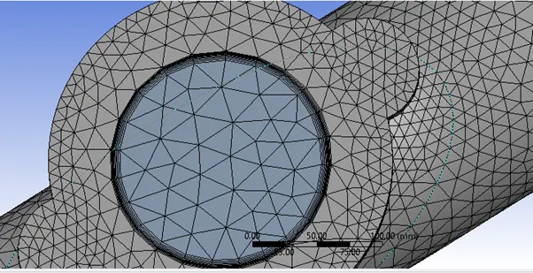
Elements=374957

Mesh size=150mm

Mesh size of convection wall volume sizing=10mm with capture curvature on.

Inflation layers=5 , thickness =5mm

3-Open setup and then File> mesh recorded operations >match zone names .

Create setup as Pressure based solver, k-epsilon model, steady mode. Material-fluid=air, material-solid=aluminium.

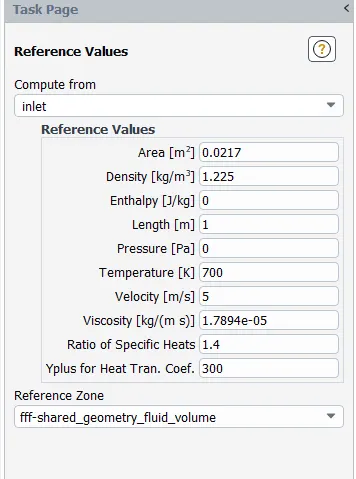
Boundary setup- Inlet=5m/s, 700K

Outer wall convection=choose convection and input the coefficient as 20W/mK .

Outlet and inflation layer need no separate editing and the extra walls in the rest of the geometry are adiabatic and we don’t need to input(heat flux=0 there) that in boundary setup or in named selection.

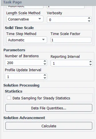
Initialize the solution, create pressure and velocity contours and create report for heat transfer coefficient. Run the simulation for 200 iterations.

4-Go to results and observe .

Q2. Justifying the value of y+ taken.

As we know the flow is turbulent, and we provide inflation layer near the wall , so basically we are focussing on the laminar region near the walls which is a part of the turbulent flow. In order to capture this small region, mesh sizing here should be small as well. To determine the size of the first cell from the wall (basically distance of wall surface to the cell node of the first layer of cell attached to wall), i.e. the y value we have the formula:

y+= yu*/v

y+=10 or less for cell node to be in the laminar region of the turbulent flow and >30 for cell node to be in turbulent region of the turbulent flow. Region between this is the transitional region.

Considering y+=10

V=5m/s

U*=frictional velocity where u*²=T/ρ

T=wall shear stress

Ρ=density=1.225kg/m³

Now, T= Cf*0.5*ρ*v²

Cf=friction coefficient=0.0576Re^-1/5

Re=ρDv/µ

D=0.166m (from space claim geometry data , we find inlet dia)

Ρ=density of air=1.225kg/m³

µ=Viscosity=1.7894e-05 kg/ms

v=5m/s

Re=56820.7

Cf=0.00644

T=0.0986 calculated from the above formula

Hence,

u*²=T/ρ

U*=0.283m/s

Hence, y=6.3mm from the formula

y+= yu*/v

Hence, any value below 6.3mm for inflation layer thickness is valid as it comes under the laminar region which is occurring near the wall(where we apply the inflation layer).

Q3. Calculate heat transfer coefficient and show the temperature and velocity contours.

Creating a report>area weighted average>wall fluxes>surface transfer coefficient for inflation layer named selection.

After running setup and computing heat transfer coefficient from the report. We get,

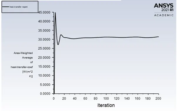
Heat transfer coefficient from Ansys fluent report: 31W/m2K

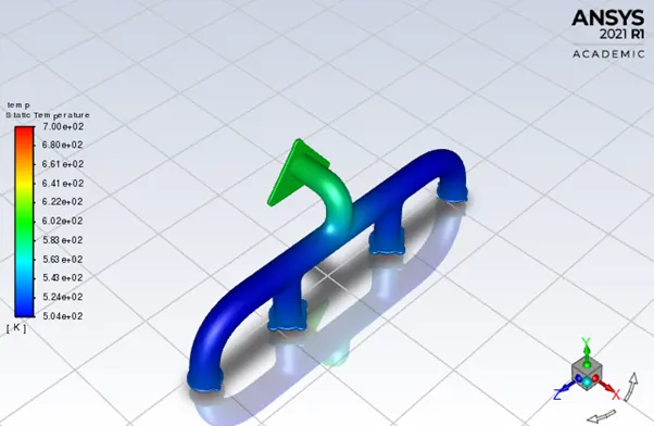
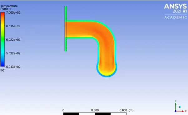
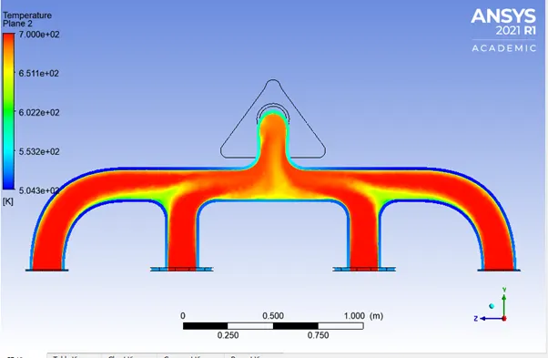
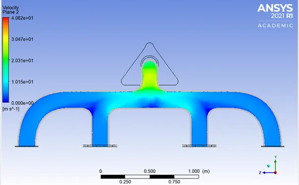
Temperature and Velocity contours:

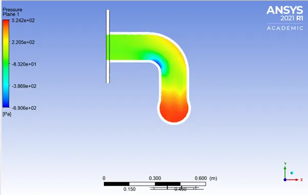
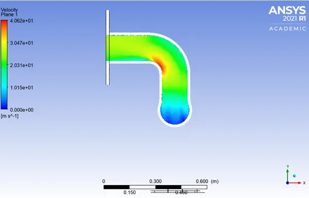
The place where pipe has bend shows the highest velocity as a higher pressure loss occurs there due to sudden change of velocity direction at the bend which exerts a force on the flowing liquid and it separates from the inner portion of bend creating a low pressure and high velocity region there.

Observations:

Residual data:

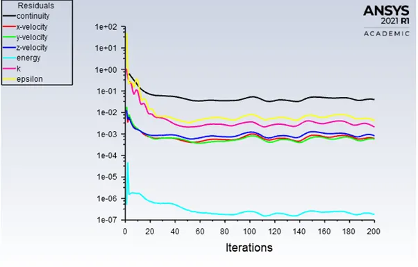
The simulation curves converges at nearly 80 iterations.

Heat transfer coefficient:

Q4. How do you verify if HTC Predictions are correct? On what factors does the accuracy of the prediction depend on?

Heat transfer coefficient from ansys fluent report: 31W/m2K

We verify value from the following relation:

Value from Dittus-Boelter correlation:

Nu=Nusselt number, Pr=Prandtyl number, Re=Reylond number

Nu=0.023Re^0.8 Prⁿ

n=0.4 for hot fluid

Valid for prandtyl no.( 7-160) and reylond number>10000,

Re=ρDv/µ

D=0.166m (from space claim geometry data , we find inlet dia)

Ρ=density of air=1.225kg/m³

µ=Viscosity=1.7894e-05 kg/ms

v=5m/s

Re=56820.7

This means the flow is turbulent, that’s why we used the turbulent model for simulation.

Pr=µCp/k

µ=Viscosity=1.7894e-05 kg/ms

k=Thermal conductivity=0.0242 W/mK

Cp=specific heat =1006.43J/kgK

Pr=0.744

Putting the two values of Re and Pr in Dittus-Boelter correlation:

Nu=129.9 i.e., 130

Nu=hL/k

k=Thermal conductivity=0.0242 W/mK

L=diameter of inlet =0.166m

h=heat transfer coefficient as per co-relation =18.9 W/m²K

Now, this value is not exactly similar to actual heat transfer coefficient from the simulation but is in the considerable range.

The accuracy of prediction depends on Prandtl number and Reynold number calculation and the factor n in the formula /correlation. A difference between theoretical and simulated values of h is thus considerable.

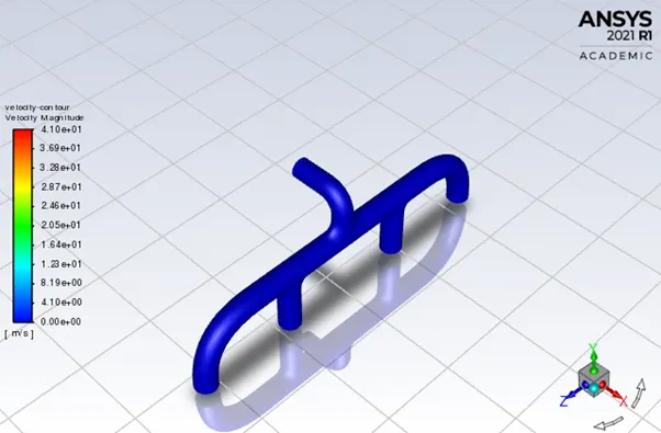
Conclusion: We can conclude that as per mass conservation principle, the velocity at outlet will be larger as the flow from 4 inlet areas exit through only 1 outlet area and hence the flow has to increase its velocity and hence the flow is having highest temperature at outlet pipe. The place where pipe has bend shows the highest velocity as a higher pressure loss occurs there due to sudden change of velocity direction at the bend which exerts a force on the flowing liquid and it separates from the inner portion of bend creating a low pressure and high velocity region there. This is also illustrated in the observations .