Week 5 - Curve fitting

Curve-Fitting challenge

The functions that we define here give relationship between cp and temperature. Where a,b,c are the co-efficient. This is a function that we think will give us best fitted curve for the actual curve (which is curve for cp and temperature). We try to try different curves.

1. What does Popt and pcov mean?

The Curve_fit function returns two items, which are Popt and pcov. The Popt argument are the best-fit parameters for a ,b& c coefficients of the function we have defined. Popt gives the best fitted values of co-efficient of the function.

The pcov variable contains the covariance matrix, which indicates the uncertainties and correlations between parameters. This is mostly useful when the data has uncertainties.

Scipy module has many functions, one of them is to optimize i.e., using curve fit data. We try to fit models to the data. Curve_fit is one such scipy routine for this.

2.What does np. array(temperature) do?

Here when we are plotting the curve fit function, we call the function and put arguments but in temperature argument We are passing temperature values in the data in the form of a collection or array. Hence, we use np.array(temperature).

3.* in *Popt means that we are referring to these Popt values that we have mentioned.

*Popt is the other argument for the function which denotes array of a,b and c co-efficient which are also necessary to call the function. Using a star value helps to refer to these values.

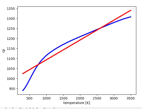
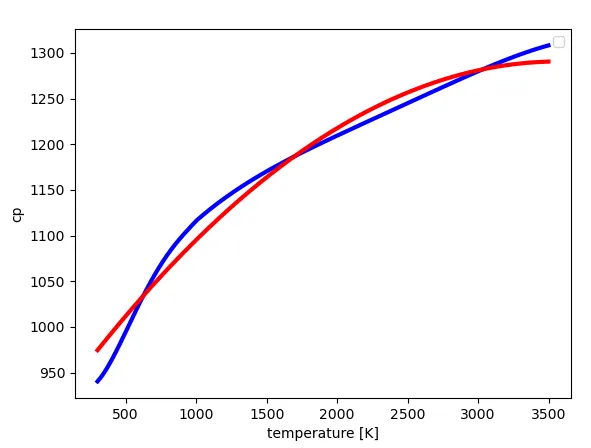
4.Write code to fit a linear and cubic polynomial for the Cp data. Explain if your results are good or bad.

Code with linear:

import numpy as np 
import matplotlib.pyplot as plt 
from scipy.optimize import curve_fit

#relationship  of temperature and cp in data values as per our opinion is defined here in this function

def func(t,a,b,c,d):
	return a*t+b
	#return a*pow(t,2)+b*t+c
	#return a*pow(t,3)+b*pow(t,2)+c*t+d
	#return a*pow(t,4)+b*pow(t,3)+d
	
def read_file():
	temperature=[]
	cp=[]
	for line in open('data','r'):
		values=line.split(',')
		temperature.append(float(values[0]))
		cp.append(float(values[1]))
	return[temperature,cp]

temperature,cp=read_file()
popt ,pcov=curve_fit(func ,temperature ,cp)
fit_cp=func(np.array(temperature),*popt)
#printing popt value for cubic function because it fits the best.
print("best fit value for a,b,c= ")
print(popt)
print("temperature array values=")
print(np.array(temperature))
print("best fit cp values evaluated from function=")
print(fit_cp)
print("actual value of cp=")
print(cp)

plt.plot(temperature,cp,color="blue",linewidth=3)
plt.plot(temperature,fit_cp,color="red",linewidth=3)
#plt.legend('actual data','curve fit')
plt.xlabel('temperature [K]')
plt.ylabel('cp')
plt.show()

Plot with linear:

Code with quadratic:

import numpy as np 
import matplotlib.pyplot as plt 
from scipy.optimize import curve_fit

#relationship  of temperature and cp in data values as per our opinion is defined here in this function

def func(t,a,b,c,d):
	#return a*t+b
	return a*pow(t,2)+b*t+c
	#return a*pow(t,3)+b*pow(t,2)+c*t+d
	#return a*pow(t,4)+b*pow(t,3)+d
	
def read_file():
	temperature=[]
	cp=[]
	for line in open('data','r'):
		values=line.split(',')
		temperature.append(float(values[0]))
		cp.append(float(values[1]))
	return[temperature,cp]

temperature,cp=read_file()
popt ,pcov=curve_fit(func ,temperature ,cp)
fit_cp=func(np.array(temperature),*popt)
#printing popt value for cubic function because it fits the best.
print("best fit value for a,b,c= ")
print(popt)
print("temperature array values=")
print(np.array(temperature))
print("best fit cp values evaluated from function=")
print(fit_cp)
print("actual value of cp=")
print(cp)

plt.plot(temperature,cp,color="blue",linewidth=3)
plt.plot(temperature,fit_cp,color="red",linewidth=3)
#plt.legend('actual data','curve fit')
plt.xlabel('temperature [K]')
plt.ylabel('cp')
plt.show()

Plot with quadratic:

Code with cubic:

import numpy as np 
import matplotlib.pyplot as plt 
from scipy.optimize import curve_fit

#relationship  of temperature and cp in data values as per our opinion is defined here in this function

def func(t,a,b,c,d):
	#return a*t+b
	#return a*pow(t,2)+b*t+c
	return a*pow(t,3)+b*pow(t,2)+c*t+d
	#return a*pow(t,4)+b*pow(t,3)+d
	
def read_file():
	temperature=[]
	cp=[]
	for line in open('data','r'):
		values=line.split(',')
		temperature.append(float(values[0]))
		cp.append(float(values[1]))
	return[temperature,cp]

temperature,cp=read_file()
popt ,pcov=curve_fit(func ,temperature ,cp)
fit_cp=func(np.array(temperature),*popt)
#printing popt value for cubic function because it fits the best.
print("best fit value for a,b,c= ")
print(popt)
print("temperature array values=")
print(np.array(temperature))
print("best fit cp values evaluated from function=")
print(fit_cp)
print("actual value of cp=")
print(cp)

plt.plot(temperature,cp,color="blue",linewidth=3)
plt.plot(temperature,fit_cp,color="red",linewidth=3)
#plt.legend('actual data','curve fit')
plt.xlabel('temperature [K]')
plt.ylabel('cp')
plt.show()

Plot with cubic:

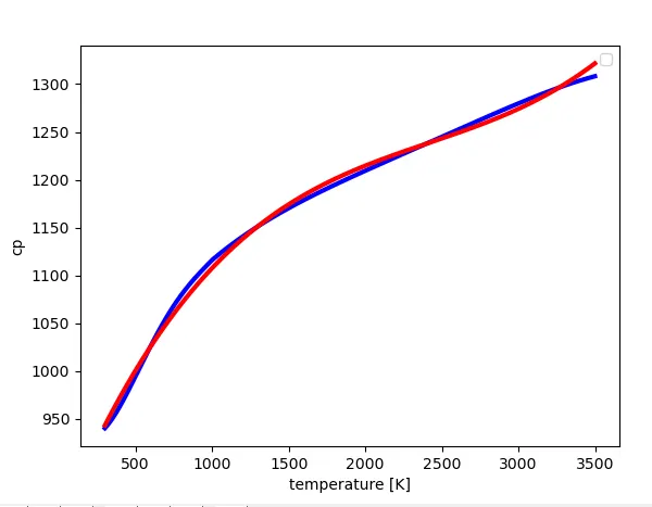
We can see cubic curve fits best. Blue is the actual curve and red curve is the best fit curve.

Code with 4 degree polynomial:

import numpy as np 
import matplotlib.pyplot as plt 
from scipy.optimize import curve_fit

#relationship  of temperature and cp in data values as per our opinion is defined here in this function

def func(t,a,b,c,d):
	#return a*t+b
	#return a*pow(t,2)+b*t+c
	#return a*pow(t,3)+b*pow(t,2)+c*t+d
	return a*pow(t,4)+b*pow(t,3)+d
	
def read_file():
	temperature=[]
	cp=[]
	for line in open('data','r'):
		values=line.split(',')
		temperature.append(float(values[0]))
		cp.append(float(values[1]))
	return[temperature,cp]

temperature,cp=read_file()
popt ,pcov=curve_fit(func ,temperature ,cp)
fit_cp=func(np.array(temperature),*popt)
#printing popt value for cubic function because it fits the best.
print("best fit value for a,b,c= ")
print(popt)
print("temperature array values=")
print(np.array(temperature))
print("best fit cp values evaluated from function=")
print(fit_cp)
print("actual value of cp=")
print(cp)

plt.plot(temperature,cp,color="blue",linewidth=3)
plt.plot(temperature,fit_cp,color="red",linewidth=3)
#plt.legend('actual data','curve fit')
plt.xlabel('temperature [K]')
plt.ylabel('cp')
plt.show()

Plot with 4 degree polynomial:

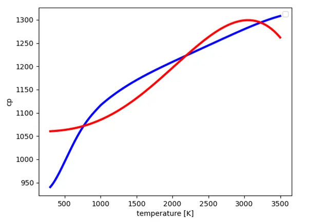
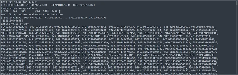
Conclusion:Here we can compare the best fit values of cp and actual value of cp, they are almost similar. This is why the curve with cubic equation fits best with the data.

5.What needs to be done in order to make the curve fit perfect?

We can see cubic curve fits best. Blue is the actual curve and red curve is the best fit curve. We need more and more values of data in order to fit the curve perfectly with the actual curve, there is a difference between the two because for curve fit plot , we only have a limited set of values.

6.Show empirically as to how well your curve has been fit.

Here we can compare the best fit value of cp and actual value of cp, they are almost similar. This is why the curve with cubic equation fits best with the data.