Week 7: Shock tube simulation project

Shock tube simulation

Shock tube is a vessel in which one part is at high pressure and other is at low pressure separated by a diaphragm. when the diaphragm is removed suddenly, a compression wave travels into the low pressure region and a expansion wave or fan at the same time propogates from the high pressure region. Between these two moving waves is a parting line which is between these two pressure regions is contact surface.The expansions are adiabatic and reversible, so they are isentropic. Shock tube are used to study high speed flows, these are very short duration experiments. They are used to find ignition delay also. The wave that travels towards the low pressure surface gets reflected back from the end and comes back and travels in opposite direction.

Waves formed in shock tube pressure regions:

Expansion wave forms in region having earlier high pressure and compression normal shock wave forms in region having initially low pressure.

Importance of shock tube:

Shock tube is used to simulate combustion models and find ignition delay.

Simulating this in converge:

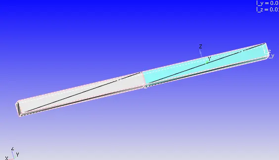
First , we create a geometry formed by two cuboidal volumes kept side by side. We create two boundaries, each boundary contains all surfaces of the cuboidal region. Also, these two volumetric regions will be used to form 2 regions. Region 1- high pressure region and region2- low pressure region.

Boundary setup-

To both the boundaries, we take the type as wall and ‘slip’ conditions as the viscosity and other gradients are low and the flow is super-sonic. In boundary 1, we give the species as nitrogen and having pressure of 6 bar. In boundary 2, we give the species oxygen and pressure as 1 bar.

Event setup-

From 0 to 0.001 seconds, the diaphragm or the connection between two regions is closed. At 0.001 seconds the connection is opened and the diaphragm is broken.

Simulation time-

The run time is 0.003 seconds with minimum time step as 1e-8.

Base grid :

Base grid taken is 0.004 with adaptive mesh refinement by ‘species’ nitrogen and using sgs temperature for nitrogen as 0.001 and the embedding level as 3.

Output files:

We take time interval for writing 3d output data files as 1e-5 and time interval for writing the text output as 1e-6.

Observations:

Geometry of shock tube , the two colors define the two regions:

Transient cell count plot:

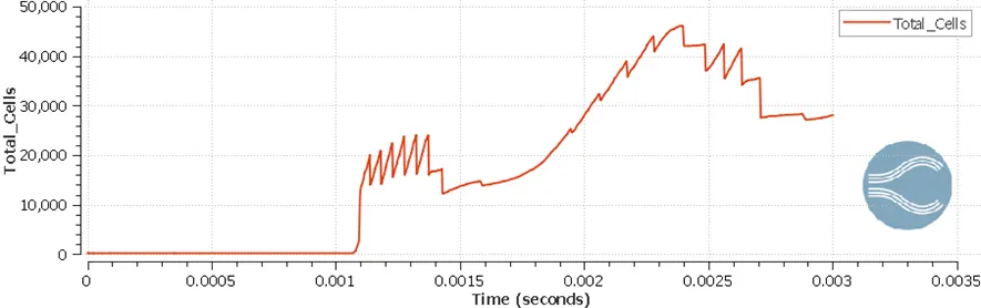
After 0.001 seconds, the diaphragm is opened and flow starts, now the adaptive mesh refined is as per the change in the species n2’s change as the gases mix, so mesh gets refined as the diaphragm opens and due to this number of cells needed increase. This can be seen in the plot for mass fraction of n2 and o2 shown below. As the change in species concentration , cell count increases i.e. now the mesh adapts to a finer mesh and as the concentration becomes stagnant , the cell count reduces or lesser number of cells are required now.

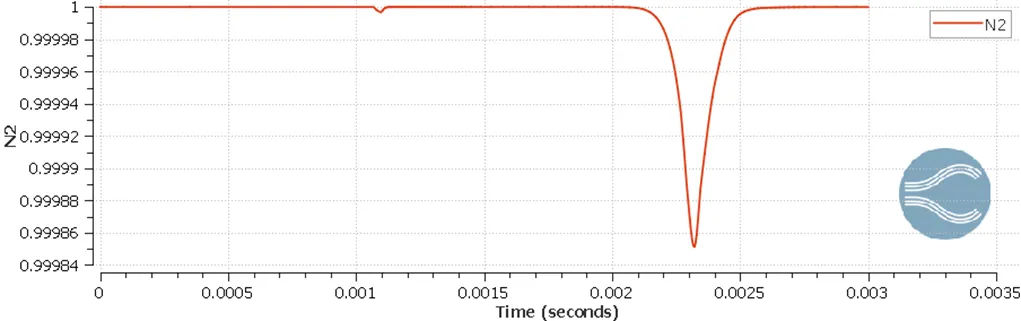
The mass fraction of n2 till 0.001 seconds is 1 because the diaphragm has not been opened up. Now at 0.001 seconds, oxygen is introduced , so there is a sudden decrease in n2 mass fraction . This is a plot of region 1 i.e the region of high pressure where only nitrogen was present before diaphragm opens and after it opens, how the content of nitrogen drops in it. Content of nitrogen will increase in it again as the wave reflects back.

Looking at the region 2 i.e. the region initially having low pressure and filled with oxygen. The breaking of diaphragm and incoming of nitrogen into that is shown as:

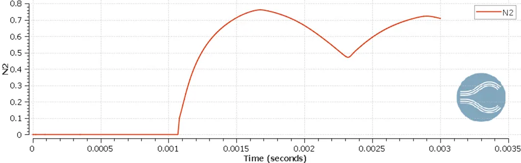
This region did not contain nitrogen earlier and after 0.001 seconds, the mass fraction increases suddenly (although this value is very low, at 0.0015 seconds, nitrogen has just occupied 0.8 mass of the total mass of region2) and as after some time the wave reflects and moves in opposite direction , that mass fraction of nitrogen introduced to that region lowers again . It will keep on rising and lowering.

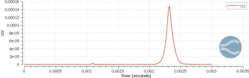
Change of oxygen mass fraction in region 1:

Pressure Vs time

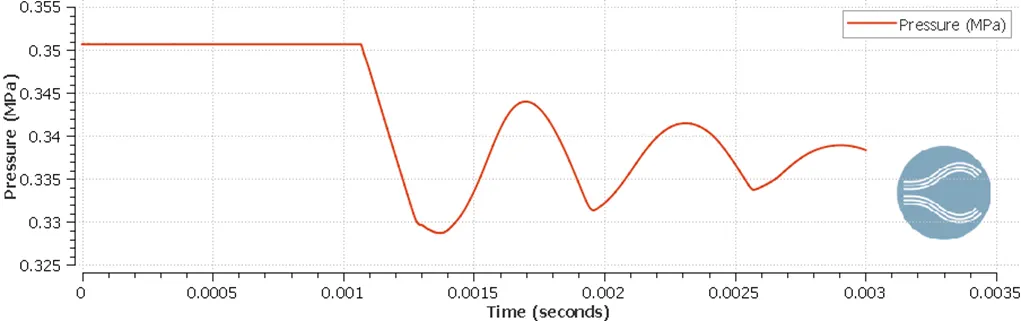
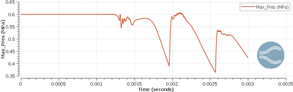
This is the pressure of the whole tube as an average. Below we can see the plot for max pressure in the tube. We have 6 bar on the high pressure side as the max pressure which then goes on reducing as the waves travel. The shock wave travels from the high pressure to the low pressure region. Due to this the pressure reduces and this wave then comes back after reflecting and collides with the mixture travelling towards the wall and forces it to stop or decreases its velocity and changes the direction. Thus the pressure increases again and then reduces , this cycle continues.

Mesh image for shock tube:

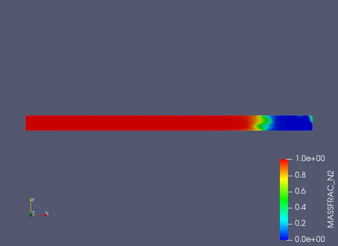
This is the image for mass fraction of nitrogen at the final time step i.e . at 0.003 seconds, we can see that mesh gets really refined in the area where the shock wave is travelling because there the nitrogen mass fraction keeps on changing.

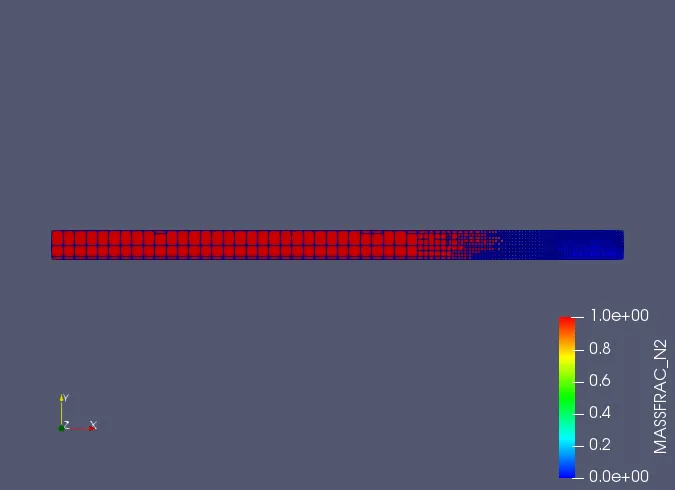
Nitrogen mass fraction image:

Temperature plot:

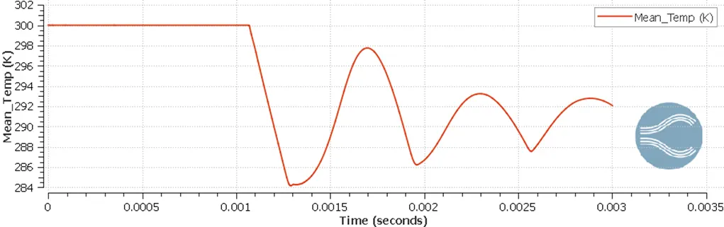
This is the plot for mean temperature. Initially, the temp is 300k and then as the pressure in the high pressure region reduce and gas expands into the low pressure region, as the pressure reduces, the gas temperature reduces due to this isentropic expansion happening. As this wave travels in the opposite direction after reflecting from the wall and compresses the region in front of it, the temperature increases again. Again , this mixtures goes on expanding in the whole region and decrease temp. Thus, this oscillating and damping sort of temperature and pressure curves are obtained.

video link:

Conclusion:

The shock tube is an important simulation to experiment the ignition delay. The results obtained are in agreement with the theortical observations. Adaptive mesh refinement is used to refine the mesh where concentration of n2 changes and the wave travels. The simulation is ran for a short time of 0.003 seconds. The results obtained are shown in the report as such.