Week 1- Mixing Tee
Mixing Tee-simulation in ANSYS Fluent
It is a device in which hot air enters from one inlet at a certain temperature and mixes with the cold air entering from the other inlet at a different temperature and finally air at the reuired temperature comes from outlet. Mixing Tee has a very useful application in air conditioners to mix the fresh air and return air. It is also used in petrochemical products and in blending of fuel gas and other oils.
Procedure:
Open Space Claim and load the respective geometry. The geometry loaded has some thickness also but it is not relevant to perform the flow simulation. Hence, we can Extract Geometry (In Prepare tab) > select edges we want to extract and apply. Now supress the solid model for physics.
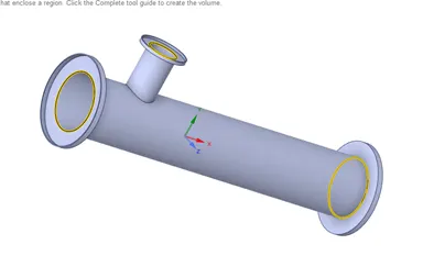
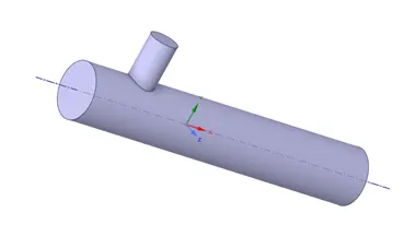
Now open Mesh module . We need 2inputs here: Element Size and named selection. Element size are inputed as per case and 4 named selection are made. They are: Walls, Inlet_Y, Inlet_X, outlet. After this mesh can be generated.
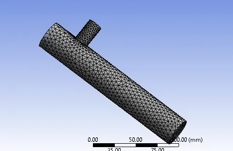
Once mesh is generated, setup for the simulation is required.
This is a steady state simulation (we are interested in the outcome) with a pressure based solver with absolute velocity formulation .Energy equations must also be solved here as temperature is of importance here.
Select the type of model (k-epsilon or k-omega as per case ).
Create a material as air.
Change units if temperature as per choice.
Create boundary zones and cell zones. Cell zone is fluid type with material as air.In Boundary zone, automatically the boundary type appears for each named selection. Input velocity of inlet in X &Y and temperature in both as per the case.
To analyse temperature value at outlet, we can select surface report for area weighted average ( definition>new> Surface report> area weighted average). Similarly , for effectiveness of mixing we can select the standard deviation report.
Go for hybrid initialization and run the iteration for 400 iterations with convergence check.
Absolute criteria for all the residual are mostly 0.001 here (except for energy for which it is 1e-6). Residual are : X, Y, z velocity, energy, continuity and turbulence variables.
Run the calculations and plot the graph.
Table of Inputs:
|
Area of Inlet-X/Outlet(mm) |
Area of Inlet_Y(mm2) |
Length of cylinder wall |
v_Inlet_X |
v_inlet_Y |
T_inlet_X |
T_inlet_Y |
Model used |
||
|
Case 1a |
Short Tee |
901.31 |
225.983 |
5.18 |
3 |
6 |
36 |
19 |
Realizable k-Epsilon with standard wall function |
|
Case 1b |
Short Tee |
901.31 |
225.983 |
5.18 |
3 |
6 |
36 |
19 |
k-omega SST |
Case 1a:
|
Type |
Mesh Size |
Model |
Momentum ratio |
|
Short Tee |
5mm |
K-Epsilon |
2 |
Case 1b:
|
Type |
Mesh Size |
Model |
Momentum ratio |
|
Short Tee |
5mm |
K-Omega |
2 |
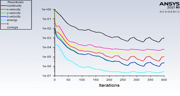
Residual Graph Comparison:
Convergence Plot:
K-epsilon model takes approx. 175 iterations.
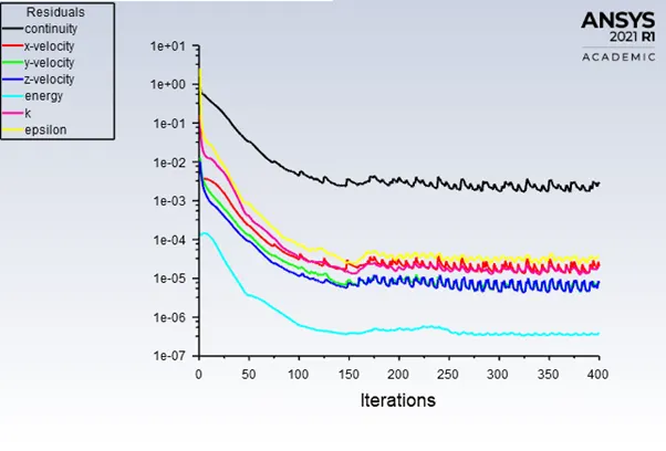
K-Omega SST Model takes 225 iterations:
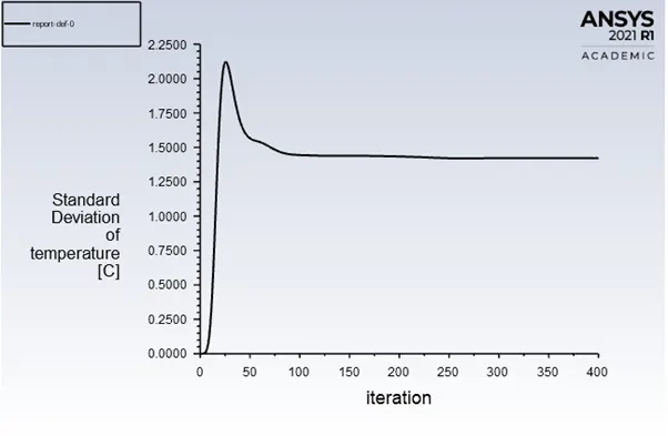
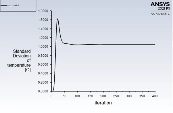
Standard deviation Curve:
k-epsilon model:
K-Omega SST model:
Observations:
K-Epsilon Temperature contour :
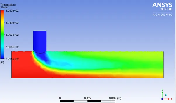
K-Omega SST Model Temperature Model:
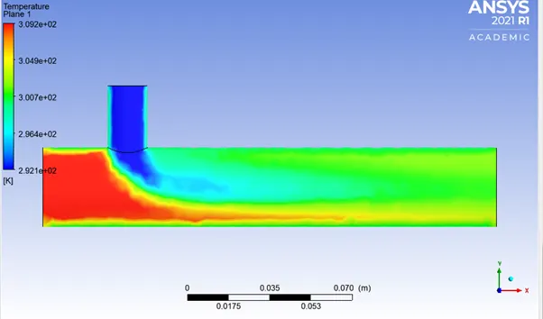
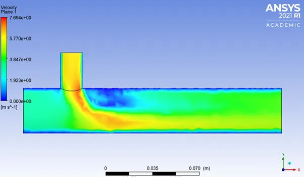
K-Epsilon Velocity Contour along Length:
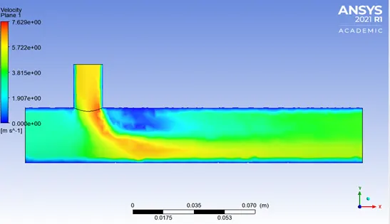
K-Omega SST Model Velocity Contour:
Line plot
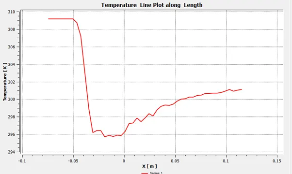
K-epsilon Temperature Line Plot along Length of Pipe:
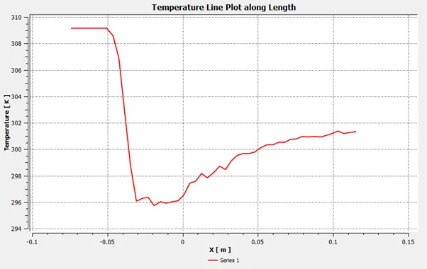
K-Omega SST Model Temperature Plot along Length:
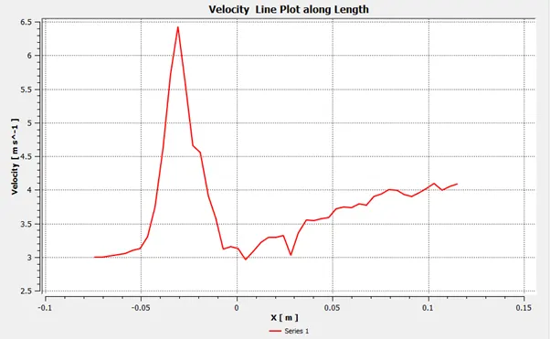
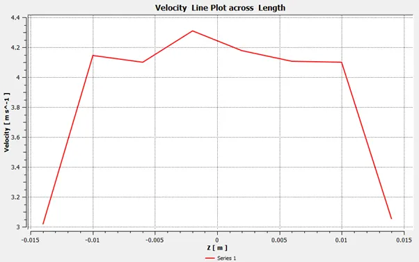
K-Epsilon Velocity Line Plot along Length:
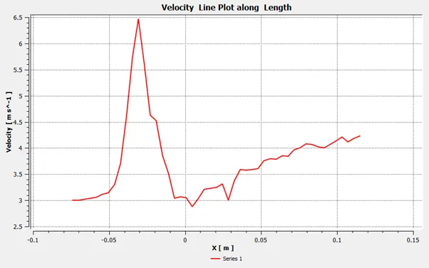
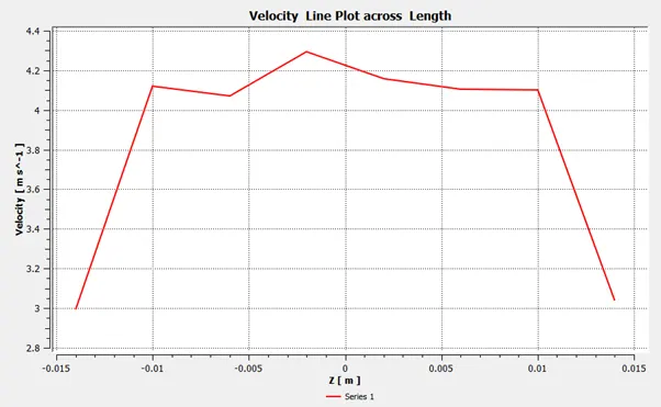
K-Omega SST Model -Velocity Line plot Along Length:
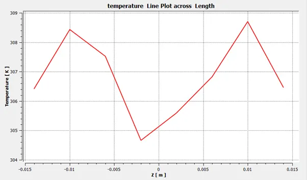
K-Epsilon model -Temperature Line Plot across Length of Pipe (Cross section):
K-Omega SST Model Temperature Line Plot across Length:
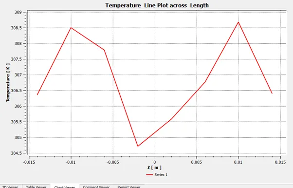
K-epsilon model-Velocity Line Plot across Length
K-Omega SST Model across Length:
Average Outlet Temperature:30.2
Formula:
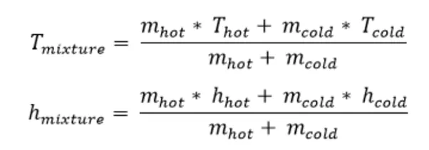
mass per sec is=area*velocity
Area of the cross sections & Velocity is given in the table above .
|
Average outlet Temp computed as per report |
30.2 |
|
Average outlet Temp Calculated |
30.32 |
Cell Count for both cases, iteration to converge and outlet area weighted temperature are provided as in the table below:
|
Mesh Size |
Cell count/nodes |
Iteration to converge |
outlet area weighted average T |
||
|
Case 1a |
Short Tee |
5mm |
3142 |
175 |
30.25 |
|
Case 1b |
Short Tee |
5mm |
3142 |
225 |
29.4 |
As the no. of iterations required for convergence taken by K-Epsilon model are much lower than K-Omega SST model, it is more suitable to use a K-Epsilon model for further cases.
Case 1c
|
Type |
Mesh Size |
Model |
Momentum ratio |
|
Short Tee |
5mm |
K-Epsilon |
4 |
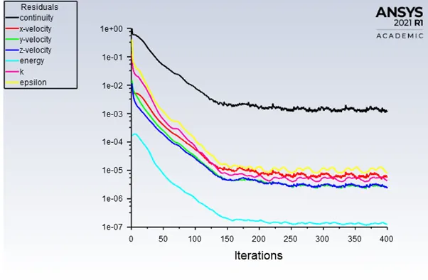
Residual Graph
Convergence at 175 iterations.
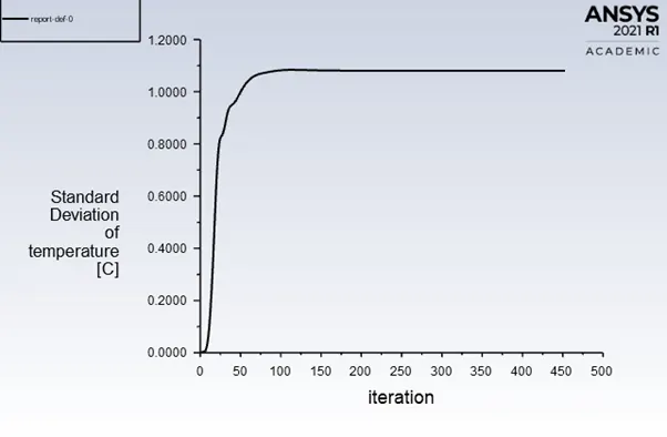
Standard Deviation :
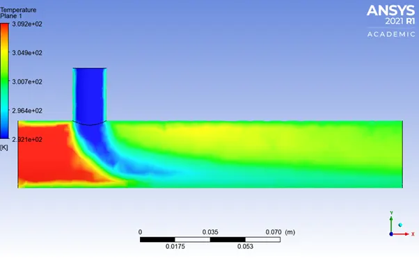
Temperature contour:
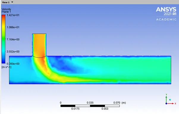
Velocity contour:
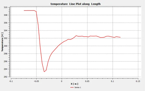
Temperature Line Plot along Length
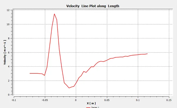
Velocity Line plot
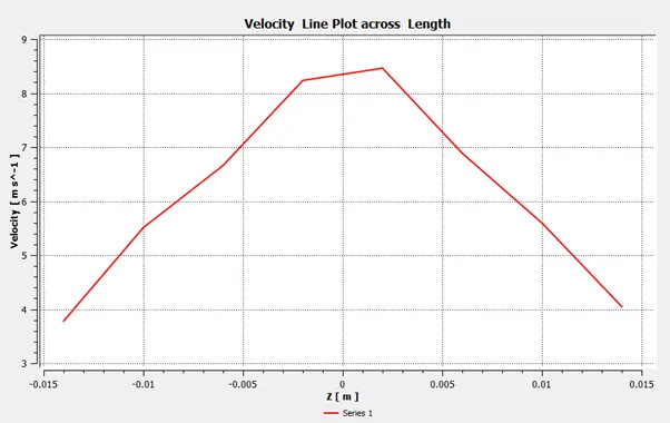
Velocity Line plot across Length
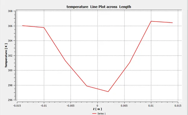
Temperature Line Plot across Length
| Mesh Size | Cell count/nodes | Iteration to converge | outlet area weighted average T | ||
| case 1 a | K-epsilon | 5mm | 3142 | 175 | 30.25 |
| Case 1b | K-Omega SSt | 5mm | 3142 | 225 | 29.4 |
| Case 1c | k-Epsilon | 5mm | 3142 | 175 | 27.1 |
Long Tee
|
Area of Inlet-X/Outlet |
Area of Inlet_Y(mm2) |
Length of cylinder wall |
v_Inlet_X |
v_inlet_Y |
T_inlet_X |
T_inlet_Y |
Model used |
Average outlet temp |
||
|
Case 2a |
Long Tee |
901.31 |
225.983 |
269.328 |
3 |
6 |
36 |
19 |
k-Epsilon |
30.32235405 |
|
Case 2b |
Long Tee |
901.31 |
225.983 |
269.328 |
3 |
12 |
36 |
19 |
k-Epsilon |
27.48765429 |
Case 2a:
|
Type |
Mesh Size |
Model |
Momentum ratio |
|
Long Tee |
5mm |
K-Epsilon |
2 |
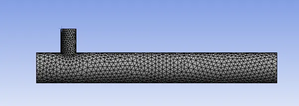
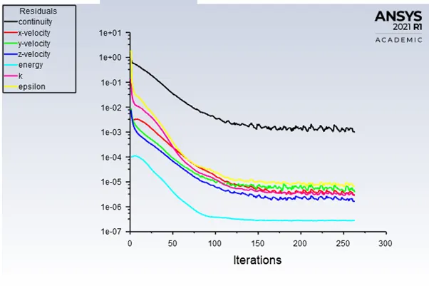
Residual Graph:
150 iterations to convergence.
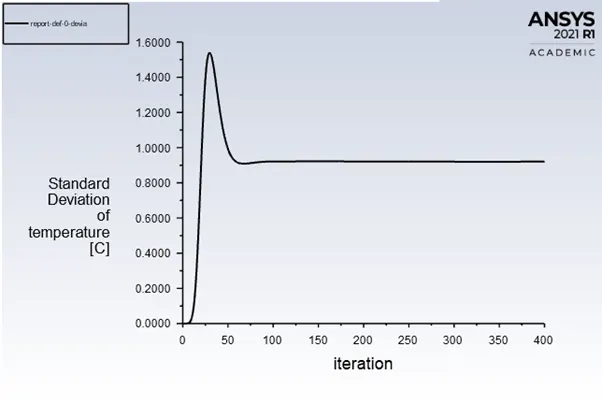
Standard deviation:
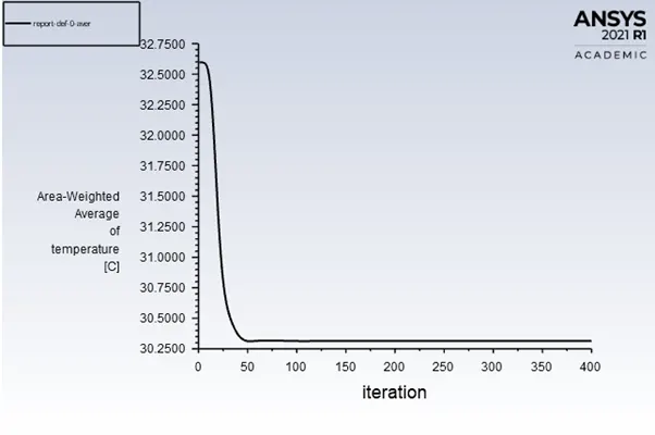
Area weighted average:
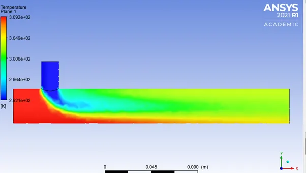
Temperature contour:
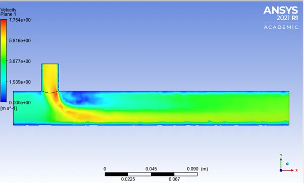
Velocity contour:
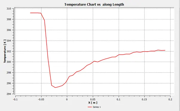
Temperature Char Along length:
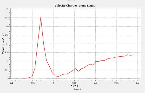
Velocity chart along Length:
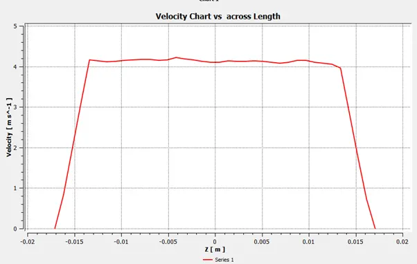
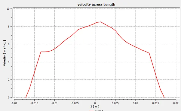
Velocity across length:
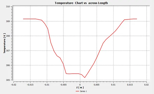
Temperature chart across length:
Case 2b:
|
Type |
Mesh Size |
Model |
Momentum ratio |
|
Long Tee |
5mm |
K-Epsilon |
4 |
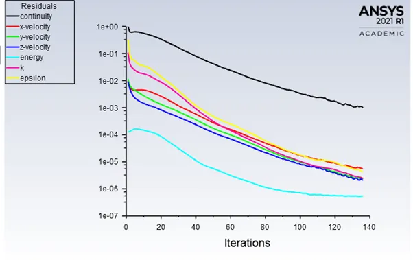
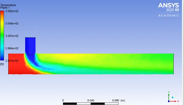
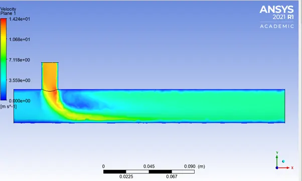
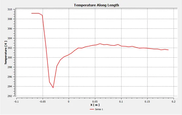
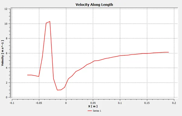
Residual:
140 iterations to convergence:
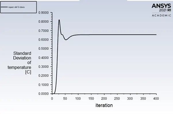
Standard Deviation
Temperature contour:
Velocity contour:
Temperature Line Plot along Length:
Velocity Line Plot along Length:
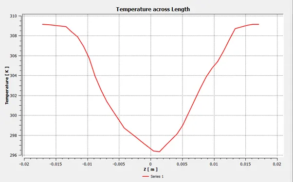
Temperature across Length:
Velocity across Length:
| Model | Mesh Size | Cell count/nodes | Iteration to converge | outlet area weighted average T | |
| Case 2a | K-epsilon | 5mm | 3936 | 150 | 30.34 |
| Case 2b | K-epsilon | 5mm | 3936 | 140 | 27.4 |
Effect of momentum ratio: Outlet temperature reduces as the momentum ratio doubles. i.e as velocity of air in the inlet_y increased , temperature at the outlet decreases.
Effect of Length: Length has no effect on final outlet temperature. The cell count increases for the same mesh size as the length increases but overall no change in temperature or no. of iterations.
Mesh Independent Study:
General Data:
|
case 3a |
Long Tee |
901.31 |
225.983 |
269.328 |
3 |
6 |
36 |
19 |
k-Epsilon |
|
Case 3b |
Long Tee |
901.31 |
225.983 |
269.328 |
3 |
6 |
36 |
19 |
k-Epsilon |
|
Case 3c |
Long Tee |
901.31 |
225.983 |
269.328 |
3 |
6 |
36 |
19 |
k-Epsilon |
Case 3a:
|
Type |
Mesh Size |
Model |
Momentum ratio |
|
Long Tee |
2mm |
K-Epsilon |
2 |
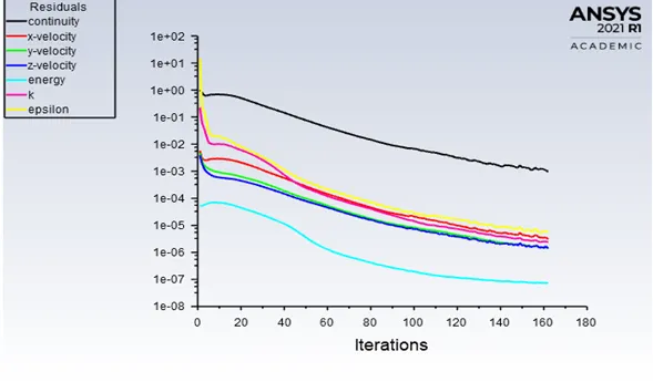
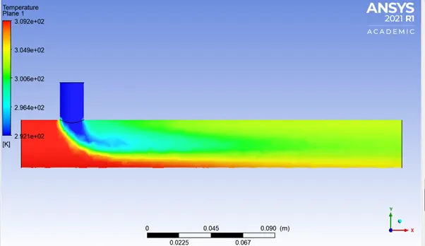
Residual Graph :
Iterations for convergence at 160 iterations.
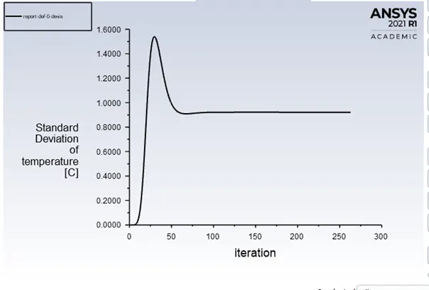
Standard deviation :
No deviation after 75 iterations.
Temperature Contour:
Temperature Line Plot along Length
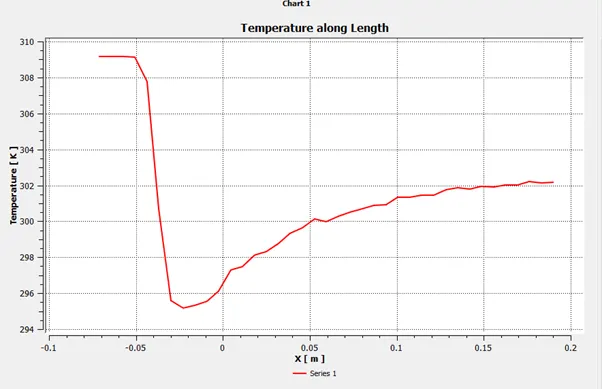
Temperature computed :30.3 degree Celsius
Case3b:
|
Type |
Mesh Size |
Model |
Momentum ratio |
|
Long Tee |
5 mm |
K-Epsilon |
2 |
Already performed before.
Iterations to convergence:280
Outlet average Temperature :30.2
Case 3c:
|
Type |
Mesh Size |
Model |
Momentum ratio |
|
Long Tee |
15 mm |
K-Epsilon |
2 |
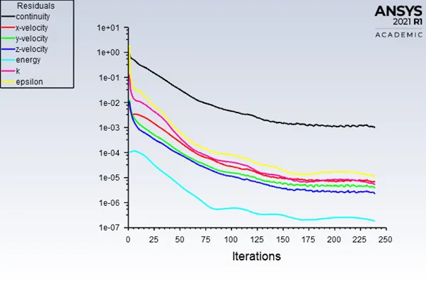
Residual Graph:
Iterations to be convergence -150 to 175
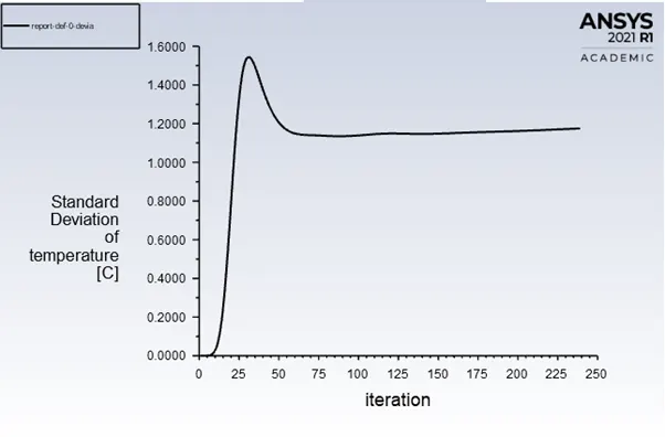
Standard deviation :
Temperature Contour:
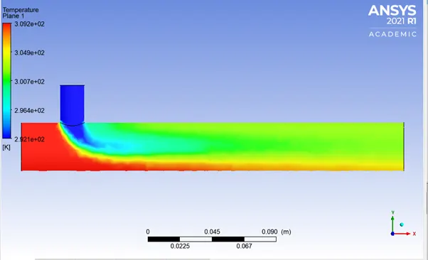
Temperature Line Plot along Length:
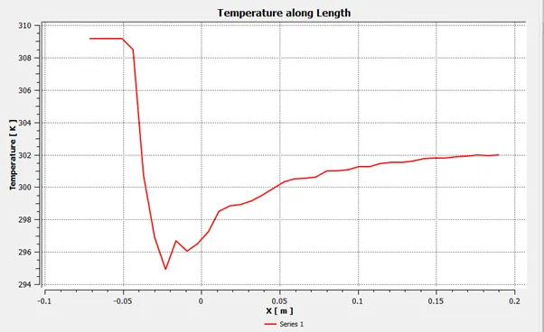
Conclusion:
|
Case |
Mesh Size |
Outlet Temperature |
Cell count |
Iterations required for convergence |
|
Case 3a |
2mm |
30.2 |
28282 |
160 |
|
Case 3b |
5mm |
30.3 |
3936 |
150 |
|
Case 3c |
15mm |
30.2 |
3432 |
150-175 |
As the outlet temperature value as well as contour does not change with change in mesh size, it can be concluded that the simulation is mesh independent. Also, the number of iterations also are almost same for every case. Hence the study is really mesh independent.