Week 3 - Solving second order ODEs

Pendulum Challenge (ODE)

Introduction: The motion of pendulum oscillation with damping can be described using simple equations. Here we try to code the co-ordinates of the mass attached to pendulum with time , create a plot for the same and create an animation for that using ‘image magick’ software. The most important part of the process is to code the change in angular displacement with time using the ODE equation concept. Here we use numpy, math, matplotlib and also from ‘scipy.integrate import odeint’.

Explanation &Procedure:

1. First, import all the required modules as mentioned in introduction.

Note the equation of motion for pendulum. This is

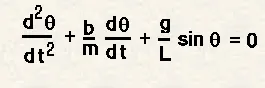
2.Convert this equation into set of ordinary differential equation. Theta1 = angular displacement

d(theta1)/dt =Theta2= velocity =

Dtheta2/dt+b/m*(theta2)+g/L*(sin(theta1))=0

This is the equation we need to solve for. For this first we create a function that returns value of differentials i.e d(theta1)/dt and d(theta2)/dt , with the help of these we find value of theta1 and theta 2 later.

B=damping coefficient=0.05

M=mass=1kg

G=gravity=9.81m/s2

L=Length of pendulum=1m

3. After doing this, we can collect all the values of theta[0] i.e angular displacement as displacement. Then run a for loop for each of this value and plot the cure for each value.

Code:

import numpy as np
import matplotlib.pyplot as plt
from scipy.integrate import odeint
import math
def model(theta,t,b,g,l,m):
	
	theta1=theta[0]
	theta2=theta[1]
	dtheta1_dt=theta2
	dtheta2_dt=-(b/m)*theta2-(g/l)*(math.sin(theta1))
	dtheta_dt=[dtheta1_dt,dtheta2_dt]
	return dtheta_dt
b=0.05
g=9.81
l=1
m=1
theta_0=[0,3]
t = np.linspace(0,20,150)
#the order of writing arguments in the ode command below should be same as that in function definition
#writing the ode
theta = odeint(model,theta_0,t,args=(b,g,l,m))
#printing the angular displacement
print(theta[:,0])

#plotting the curve of angular displacement and angular velocity with time
plt.figure(1)
plt.plot(t,theta[:,0],'b-',label=r'$\frac{d\theta1}{dt}=\theta2$')
plt.plot(t,theta[:,	1],'r--',label=r'$\frac{d\theta2}{dt}=-\frac{b}{m}\theta2-\frac{g}{L}sin\theta1$')
plt.xlabel('time')
plt.ylabel('plot')
plt.show()

#putting all the angular displacement values in a displacement array.

displacement=theta[:,0]

#for animation purpose
x0=0
y0=0
ct=1
#running a for loop to plot a separate graph at every plot and also saving  it

for value in displacement:
	x1=l*math.sin(value)
	y1=-1*l*math.cos(value)
	filename=str(ct)+ '.png'
	ct=ct+1
	plt.figure()
	plt.plot([x0,x1],[y0,y1])
	plt.plot(x1,y1,marker="o",markersize=15)
	plt.xlim(-1,1)
	plt.ylim(-1,0)
	plt.grid()
	plt.savefig(filename)

Result: Creating animation with help of image magick .

Plot of angular velocity and angular displacement w.r.t time.

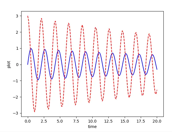
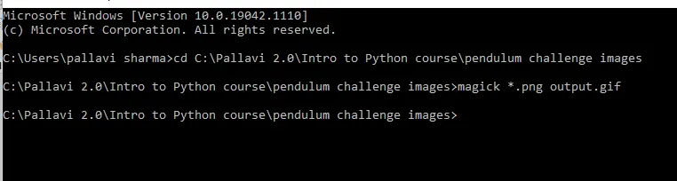
Image magick command:

Animation Link:

https://youtu.be/fgv7E1YCw2E

Conclusion: We can see the pendulum motion. Errors like indentation error, and wrong sequencing of arguments in function definition as in the ode equation. We generated 150 snaps and then created an animation out of it. Hence we can code this simualtion easily using python code.