Week 4: Project - Steady state simulation of flow over a throttle body
Steady state simulation of flow over a throttle body
As soon as the geometry of the elbow is imported in converge, diagnosis check is run in order to check for errors if any present. Here the elbow geometry consists of some thickness which we actually do not require for our simulation. So,
Step1: Automatic boundary creation: Create automatic boundary fence regions, then delete the thickness of the elbow, so that only a single surface remains.
Step-2 Repair the inlet and outlet passages: Repair has a ‘patch’ option which when applied to the open edge at inlet and outlet will patch the edge.
Step-3: Again, run the diagnosis check by clicking on find, if there are no errors, click on ‘clean’ also. Also tick the box for ‘check all the normal that are pointing to the interior ‘. After doing this, display the normal once to check if the fluid flow is inwards. in the pipe.
Setp-4 Create boundaries: Once the errors are removed, create boundaries by going in boundary option and choosing flag and ‘add ‘for inlet, outlet, elbow and throttle and assign the respective areas in the boundaries. We can also hide /unhide selected boundaries by ticking/unticking the boundary check box in the ‘view options’ column on right side.
Step-5 Case-setup: Once all of this is done, then case -setup should be done. It consists of many important steps. It sets the particular parameters for the particular simulation.
Case set-up
Click the geometry bounding box in ‘options’ to find the dimensions of the geometry. Converge assumes the file to be in metres. If the geometry is made initially in mm, then it needs to be scaled in converge. Transform consists of scale option where we have to scale the geometry to 0.001.
First: Select the time-based solver. Air as the fluid flowing. Solver type should be steady state solver with unshared memory and also set up the steady state monitor. In steady state monitor set-up, we choose the parameters for which the output we want. i.e. select average velocity, total pressure, average density at the output. For all of these we need a sample size, which is here taken 100. This means that a collection of 100 cycles is clubbed to generate average output periodically. Relative tolerance of 0.01 is taken for the case.
Second: For steady state simulation, the run time is in cycles. So,
End time-15000 cycles
Minimum time step- 1e-9
Maximum time step- 1e-9
Maximum CFL limit: always lesser than 1 i.e. here 0.5 can be taken.
Third: Region and installation – add the region and drag all the boundaries created (from view options) into the region column. Now go to the ‘boundary’ set-up and choose the following:
Inlet: Type- inflow
Pressure-1.5 bar
Temperture-300K
Fluid-air
Outlet- type- Outflow
Pressure- 1bar
Temperature- 300k
Fluid-air
Throttle- type- wall
Stationary , fixed boundary
Elbow- Type- wall
Base grid:
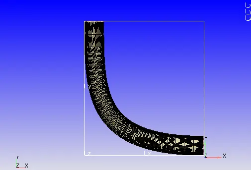
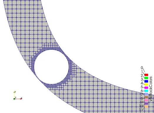
Mesh grid size of 2mm was chosen optimum here and fixed embedding for cells created near the throttle is done, so that cells near throttle become smaller in size, here they are scaled to level of 2 i.e. basically 2-time reduction by a factor of 2. There is very less area near the throttle because almost all the area in that region is occupied by the throttle and hence, a smaller number of cells are accommodated there, so in order to refine the mesh, those cells are decreased in size. This increases the cell count overall. Mesh defining is the most important part of this case setup.
Fourth: For physical modelling, the rng k-Ɛ model is selected. No changes are made in output files and post variable selection except selecting the species oxygen and nitrogen.
Fifth: After case-set-up, Export the files to a folder and run the simulation in Cygwin.
Sixth: After the simulation is run, results are post processed in converge and then opened in Para view.
Seventh: Open Para view, inside the multiblock inspector adjust the transparency of the elbow portion so that the throttle becomes visible.
CONCEPT/EXPLANATION OF THE FLOW:
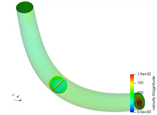
While the fluid (air here) moves through the inlet with a slightly higher pressure and the throttle is kept steady i.e. the position of throttle does not change. Here throttle acts as an obstruction to the flow. The flow as soon as it hits the throttle wall, strikes it and basically divides its path into an upper flow and lower flow, i.e. above and below the throttle (which is a disc like element placed in the pipe generally to regulate and control the flow). This helps creates a separated area like region in the mid region where fluid strikes, thus creating a region of low velocity there. Velocity is higher in the portion where the fluid passes through the tiny passage between the throttle wall and the pipe wall. This is a region of low pressure i.e. As the flow reaches the throttle valve, it faces decrease in the area of flow passage between the pipe wall and the throttle wall. So, velocity of flow increases because the area decreased. Due to this increase in velocity, as per Bernoulli theorem, the net energy should be conserved. So, to compensate kinetic energy, the pressure of the fluid decreases slightly. When the flow leaves the throttle, the pressure again increases to some extent because the area of pipe again increased which leads to decrease in velocity. For the portion on the surface of the throttle, the velocity drops at the region where the flow travels towards the outlet from the cylinder portion in the throttle because of a similar so-called separated region. The velocity is higher on the mid-surface of the cylinder in the throttle face because that cylinder portion created a region of lesser area passage for the fluid flow than it surroundings.
So, the pressure decreases around the throttle and then again increases to atmospheric pressure. It does not reduce lower than atmospheric pressure while it flows through the throttle. Velocity increases as the flow passes the throttle and again decreases as the flow has passed towards the outlet.
Mesh image:
Observations:
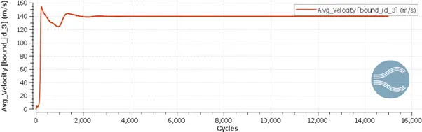
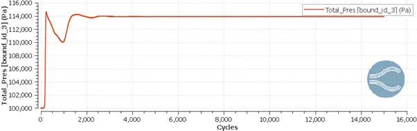
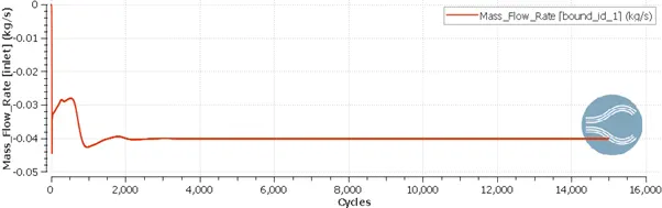
Output line plots for velocity, pressure, mass flow rate output, cell count rank
Velocity:
Pressure:
Mass flow rate input:
Mass flow rate output:
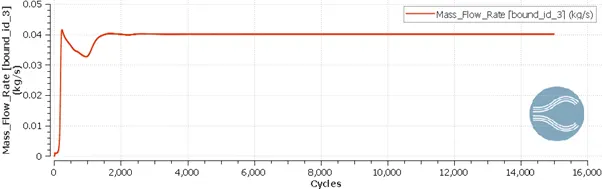
The mass inlet and outlet become constant after a certain number of cycles. The mass flow rate increases for the output and then converges and become constant. The mass flow rate for input decreases and then converges after certain cycles. The change in the rate is so steep because it takes place suddenly and then goes on converging.
The pressure and velocity output goes on converging after almost 2000 cycles. The simulation is run for 15000 cycles.
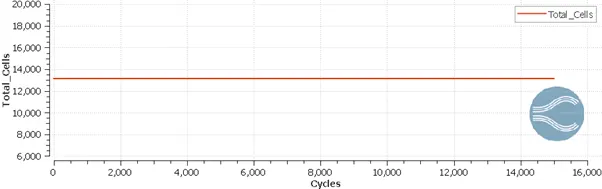
Cell count:13142 is the cell count.
Post-processed image:
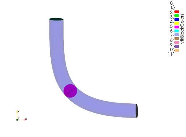
Here, the throttle is clearly visible. The elbow is shaded and inlet and outlet is also visible here.
Refined mesh image with scaled mesh size near throttle:
Pressure contour at the end of cycle;
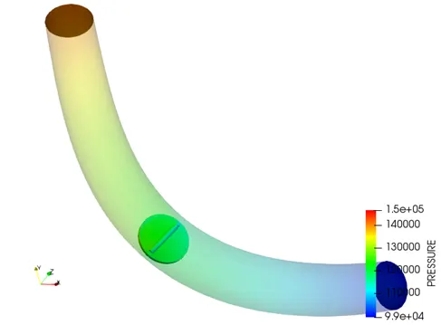
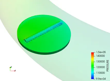
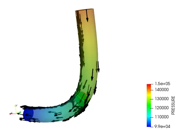
Initially the pressure is high at inlet side, after that as the flow arrives the throttle the pressure decreases as due to valve plate the velocity has increased. Pressure decreases to some value(still greater than atmospheric outlet pressure value) and decreases even more at the cylinder portion mid surface region (because there the area for flow is least technically and velocity is highest) .As the flow leaves the throttle and reaches the outlet it decreases as now, the pressure becomes same as the atmospheric pressure. At the side where the fluid flows between the pipe wall and the throttle , the area being the smallest makes the velocity higher in that region , thus increasing the pressure in that area.
Velocity contour at the end of the cycle:
Throttle detailed pic for velocity contour at the end of cycle:
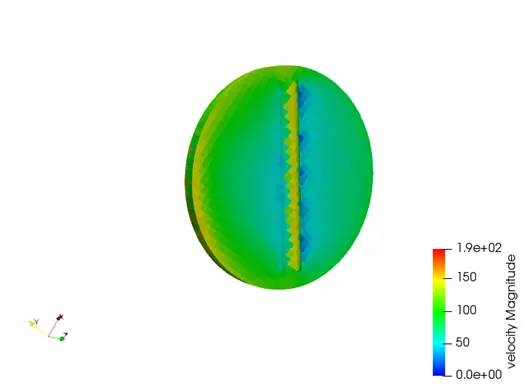
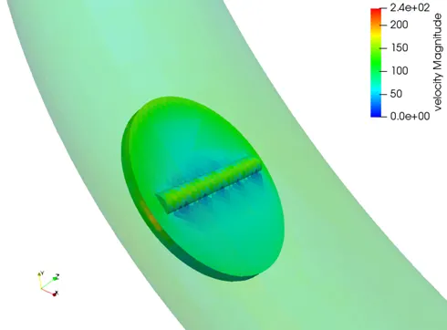
We can observe that at the end of the simulation, velocity contour for the throttle is given. As the flow reaches the throttle it separates in nearly two streams that go above and below the throttle. This creates a stagnation point at the front of the throttle. When the fluid leaves the throttle valve, then the two streams meet and similarly a separation area also occurs at the back of the throttle. Thus, the velocity drops at the front and back of the throttle. As the liquid moves over the cylindrical portion on the throttle, the velocity is increased at the mid surface of the cylindrical portion. As the flow proceeded over the cylinder and meets the surface of throttle, some flow sort of separates (this is just physically separating) and thus as we can observe in the picture above the velocity drops in the area just near the cylinder because of this. Also, at the side of the throttle, there is much less area between the pipe and the valve face for the liquid to flow and hence, the velocity drops in that region too. After the flow has passed through the throttle , it proceeds normally.
Detailed image of the throttle:
Inlet above and outlet below in the image. The liquid stream leaves the surface after it hits the cylindrical portion and that is why velocity is lower in that portion on the outlet side of the throttle.
Glpyh image:
Stream tracer :
50-100 points are taken whose paths /streamlines are traced here and the color change is w.r.t velocity.
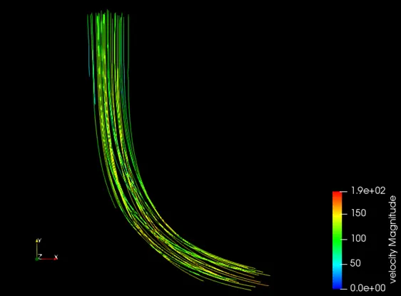
Conclusion: Thus, the flow of fluid over a steady throttle has been simulated. The results agree with the theoretical knowledge and hence are found to be correct. Actually, the velocity of particles would be zero technically which touch the surface of the throttle and hence velocity contour is supposed to be nil at the throttle but this here which converge shows is the velocity contour for the nearest cells on the pipe region above this throttle and in a way that flow is projected. Stream tracer lines are also shown which describe how the streamlines move from inlet to outlet here and the color change describes the velocity changes. Throttle is basically used to control and regulate the flow in the passage for e.g. In engines inlets to control the amount of air going in or the amount of fuel going in.
Velocity animation link :
Pressure animation link: