Week 5: Prandtl Meyer Shock problem
PRANDTYL-MEYER SHOCK FLOW PROBLEM
Case -setup:
First, diagnosis check is done and units of the geometry are checked. After that , in case setup:
Steady state solver is used here with run time for 25000 cycles where minimum time step is 1e-9. Steady state monitor set-up and region installation with 680m/s as the initial velocity 9which makes Mach no. as 2) is done as usual.
Boundaries are defined as inflow , outflow for the inlet and outlet respectively . top and bottom are wall and front and back are 2D.
The boundary conditions for inflow and outflow are already explained in the below section. After the boundary set-up, mesh size is mentioned as 0.8 here with adaptive mesh refined using temperature. Here when the sub grid scale temperature varies i.e. the derivative of temperature w.r.t flow direction more than a value 0.05 K (which we input) , then the mesh will get refined . The maximum embedding level used is 2 here which is shown under the observations.
Basic output and post variable selection is done in the regular manner and nothing is changed specifically here.
Observations with explanation and concept:
PRANDTYL-MEYER EXPANSION FAN
When a fluid has Mach number>0.3, it becomes compressible. This means now the density will no more be constant, and can change from one location to other. Here we have a duct with a sharp corner on one side. Fluid flows from this duct with supersonic speed, this means Mach number >1. The flow of fluid through this duct is isentropic if we see closely. There is no exchange of heat from the flow, so the flow is adiabatic and there is no dissipation of energy. The flow is inviscid; thus, flow can be said as reversible. This means that the flow is both reversible and adiabatic and hence isentropic. For an isentropic flow, the pressure changes proportionally as the density changes. Here because the duct expands, the fluid gets more space to fill for the same amount of fluid. So, the density of fluid decreases in order to accommodate this. The pressure also decreases due to this isentropic flow as the density has decreased. This means that as the gas expands here, the pressure, density, temperature decrease. As the pressure has dropped, this will create a faster velocity for the fluid to flow. so, velocity of fluid has increased.
As the supersonic flow encounters changes in this static pressure, the Mach waves are created at the corner. This are basically infinite shock waves which are very weak in strength as compared to an actual shock wave. The angle that these waves created with the direction of flow is µ i.e. Mach angle. sinµ=1/M where M is the Mach number. Thus, as the Mach number change (as the velocity change), we get different waves at different angles. These waves are like a disturbance which create variations in T, P, Density etc. in the flow.
WHAT ARE SHOCK WAVES?
When an object travels through a fluid, it creates disturbance which travels with a speed of sound across all directions. When an object travels with supersonic speed, its speed is higher than the speed of disturbance it creates. So, by the time disturbance travels a certain distance, the object has already travelled ahead. In supersonic flows, the fluid is not forewarned about the object. After the object has travelled, the disturbance is felt. This is a shock wave. A expansion wave is the infinitely weak shock wave that is created. It is the sound of thud that we hear when airplane with supersonic velocity travels in sky. The tangent of these disturbances created behind the object is a Mach wave and this cone formed behind the object is a Mach cone. Shock waves are of types namely, normal shock wave in which shock wave is perpendicular to the direction of flow and oblique shock wave where the wave is at some angle to the flow direction. Shock wave are an integral part of supersonic flows. These Mach waves are actually the characteristic lines at each point. In expansion fan there is disturbance and irregularity because of accumulation of many Mach waves at the same sharp corner before the expansion.
Velocity at final time step:
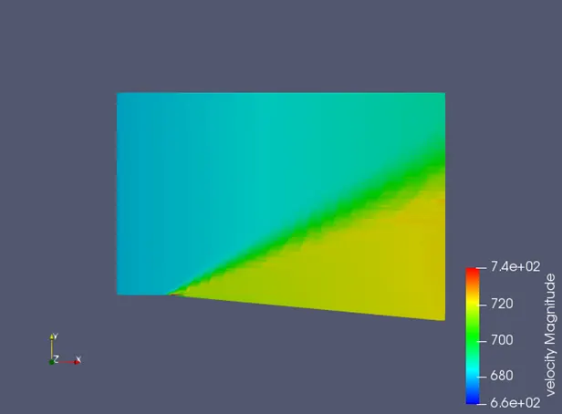
This here shows the velocity variations occurring due to the disturbance. The velocity initial was specified as 680 m/s which then goes on increasing and across the line of disturbance to the outlet it witnesses increases velocity.
Pressure at final time step:
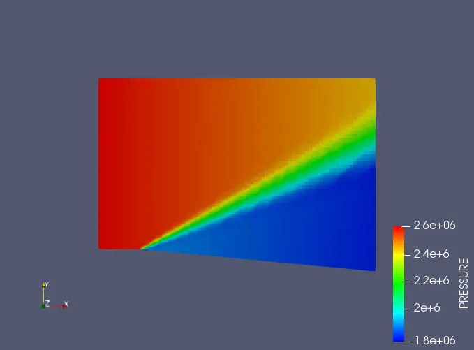
The pressure goes on decreasing as the expansion occurs and the crucial part of this variation occurs at the disturbance area after which the pressure slightly reduces. Various different pressure zones are created as a result of the disturbance.
Temperature at final time step:
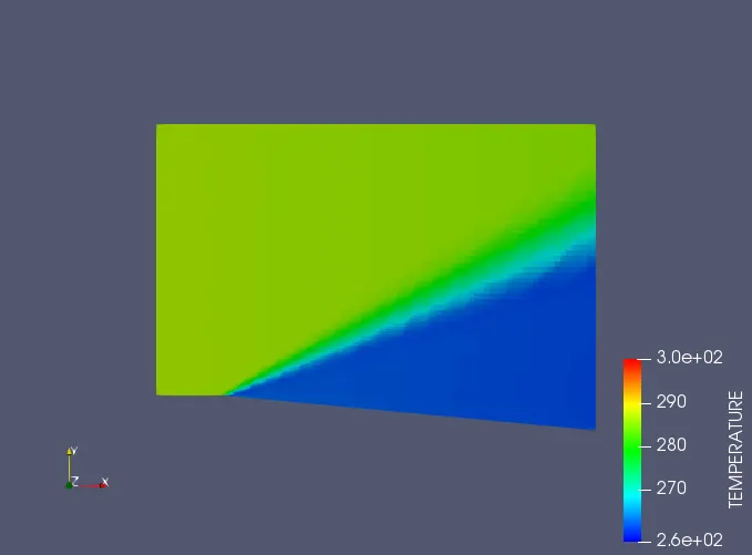
Temperature also witness sharp variations in its value. It goes on decreasing as the expansion occurs. This variation is abrupt because of the disturbance created by the Mach waves. In converge, we see the sub grid scale temperature which is derivative of temperature with position. This slope value goes on changing as the flow proceeds because of the expansion and thus, because of this, as this change is greater than 0.05K , we see the variation in mesh size also.
Close picture for temperature mesh:
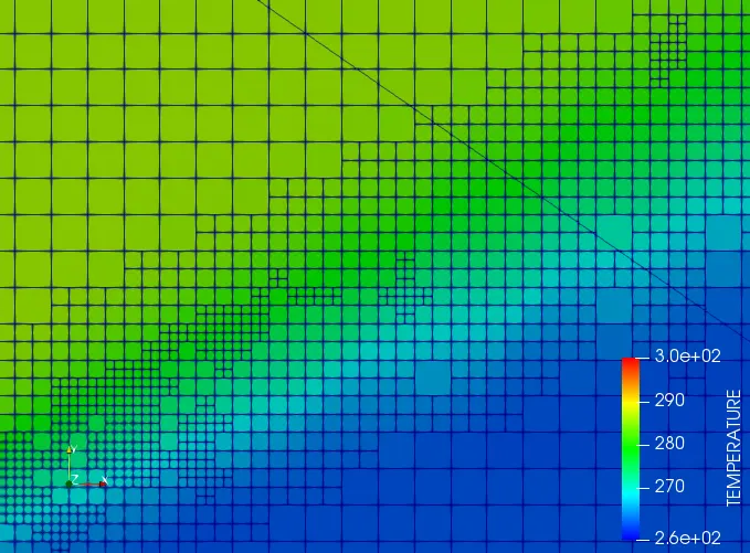
We can witness how the meshes are scaled by level of 2 (i.e. divided and made small in size) every time.
Effect of sgs(sub-grid scale temperature) parameter:
The mesh refinement occurs here when a change of 0.05k occurs in sgs , which is very small i.e. mesh refinement will be sensitive to change very much. The mesh refines after every change of sgs i.e. variation in the slope of temperature w.r.t flow direction , the mesh gets refined( here by a level of 2). By this, we can generate finer mesh at areas that change with respect to temperature or pressure or other parameters.
Cell count: Approximately 7000 cells are required.
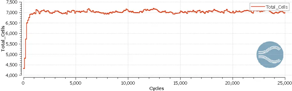
As we decrease the sgs value, i.e. if we refine the mesh even at values lower than 0.05K change, then we make the mesh even more finer. A finer mesh would require more no. of cells and hence the number of cell count will increase if the sgs value is decreased in order to make mesh finer.
Why do we choose a Neumann boundary condition for the flow here .
Here we let the boundary conditions be floated i.e. solved as the part of solution instead of giving a specified value to the variable. This can be understood as follows:
The flow here is inviscid, steady, supersonic which is a case of hyperbolic partial differential equation. The flow field is hyperbolic here and the hyperbolic equation have 2 real and distinct characteristic lines. These are the lines where the derivative of the dependent variables i.e. the solution of the pde is basically indeterminant i.e. the derivative are indeterminant at these lines. If 2 characteristic lines are emerging from any point P, then information at point P influences only the region between these characteristic lines in the direction of flow. I.e. this is the domain of influence.
These characteristic lines are the weak Mach wave at every point of this flow.
At the inlet, one characteristic line goes into the domain, so we need a stipulated specified boundary condition at that point as per method of characteristics. So, we take a velocity inlet value here(680m/s). The other characteristic lines go out of the domain, so we need to give a floating value here I.e. Neumann boundary condition is given for pressure.
At the outlet, both characteristic lines go out of the domain, hence both value of boundary conditions there are floating i.e. for both velocity and pressure the Neumann boundary condition is used. This is the input given to the boundary case-set up in converge.
Line-plotting curves:
Mass output:
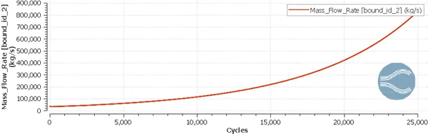
Animation link:
Conclusion: This here was a case of inviscid, steady, supersonic flow which demonstrates a hyperbolic governing partial differential equation with 2 real and distinct characteristic lines at each point. The results of the simulation are in agreement with theoretical deductions. The supersonic flow always has a shock wave/ Mach wave associated with it. The flows are compressible and the simple Bernoulli does not apply here. The change of velocity is not just dependent on area here but also the density variation in this compressible flow. The change in flow conditions by the disturbance created is shown accurately in the simulation images given.