Week 4 - Genetic Algorithm
AIM :
- To write the code in matlab to optimize the stalagmite function and find global maxima of the function
- To explain the concept of genetic algorithm and the syntax for ga in matlab
- To plot the graph of all the three studies and also for global maxima.
STALAGMITE FUNCTION
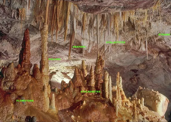
Stalagmites are formed in caves due to due to deposition of calcium carbonate and other minerals which are precipitated from mineralized water solutions. It occur under certain conditions and pH.
Stalagmite functions are mathematical functions which represent shapes similar to stalagmite.
GENETIC ALGORITHIM
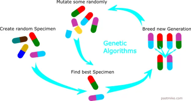
Genetic algorithim is an optimization technique for solving both constrained and unconstrained problems based on natural selection process that follows Charles Darwin theory of evolution. The algorithim repeatedly modifies a population of individual solution. During each step individuals are selected randomly from the current population by genetic algorithim which uses them as parents to produce children for the next generation. During the course of time, the population evolves towards an optimal solution.
PROCESS OF NATURAL SELECTION
clear all
close all
clc

%defining the search space
x=linspace(0,0.6,150);
y=linspace(0,0.6,150);

% creating a 2dimensional mesh
[xx yy] = meshgrid(x,y);

%evaluaitng the stalagmite function
for i=1:length(xx)
    for j=1:length(yy)
inputvector(1)=xx(i,j);
inputvector(2)=yy(i,j);
f(i,j)=stalagmite(inputvector);
    end
end

surfc(xx,yy,f)

shading interp

[input,fval]=ga(@stalagmite,2)

function[f]=stalagmite(inputvector)

x=inputvector(1);
y=inputvector(2);
f1=(sin(5.1*pi*x+0.5))^6;
f2=(sin(5.1*pi*y+0.5))^6;
f3=exp(-4*log(2)*(x-0.0667)^2/0.64);
f4=exp(-4*log(2)*(y-0.0667)^2/0.64);
f=(f1*f2*f3*f4);
end


clear all
close all
clc

x=linspace(0,0.6,150);
y=linspace(0,0.6,150);
numcases=50;

%creating a 2dimensional mesh

[xx yy]=meshgrid(x,y);

tic
%evaluating the stalgamite function

for i=1:length(xx)
    for j=1:length(yy)
    %to get x and y values
    inputvector(1)=xx(i,j);
    inputvector(2)=yy(i,j);

    %function definition
    f(i,j)=stalagmite(inputvector);

    end
end
%study 1 - statistical behaviour
for i= 1:numcases
[input, fopt(i)] = ga(@stalagmite,2);
        xa(i)=input(1);
        ya(i)=input(2);
end

time=toc;

%plotting1
figure(1)
subplot(2,1,1)
hold on
surf(x,y,f)
shading interp
plot3(xa,ya,fopt,'marker','o','markersize',5,'markerfacecolor','g')
title ('Unbounded inputs')
subplot(2,1,2)
plot(fopt)
xlabel('Iterations')
ylabel('function minimum')

function[f]=stalagmite(inputvector)
x=inputvector(1);
y=inputvector(2);
f1=(sin(5.1*pi*x+0.5))^6;
f2=(sin(5.1*pi*y+0.5))^6;
f3=exp(-4*log(2)*(x-0.0667)^2/0.64);
f4=exp(-4*log(2)*(y-0.0667)^2/0.64);
f=-(f1*f2*f3*f4);
end


clear all
close all
clc

x=linspace(0,0.6,150);
y=linspace(0,0.6,150);
numcases=50;

%creating a 2dimensional mesh

[xx yy]=meshgrid(x,y);

tic
%evaluating the stalgamite function

for i=1:length(xx)
    for j=1:length(yy)
    %to get x and y values
    inputvector(1)=xx(i,j);
    inputvector(2)=yy(i,j);

    %function definition
    f(i,j)=stalagmite(inputvector);

    end
end
tic
%study 2 - statistical behaviour - with upper and lower bounds
for i= 1:numcases
[input, fopt(i)] = ga(@stalagmite,2,[],[],[],[],[0;0],[1;1]);
        xa(i)=input(1);
        ya(i)=input(2);
end

time=toc;

%plotting
figure(2)
subplot(2,1,1)
hold on
surf(x,y,f)
shading interp
plot3(xa,ya,fopt,'marker','o','markersize',5,'markerfacecolor','g')
title ('bounded inputs')
subplot(2,1,2)
plot(fopt)
xlabel('Iterations')
ylabel('function minimum')

function[f]=stalagmite(inputvector)
x=inputvector(1);
y=inputvector(2);
f1=(sin(5.1*pi*x+0.5))^6;
f2=(sin(5.1*pi*y+0.5))^6;
f3=exp(-4*log(2)*(x-0.0667)^2/0.64);
f4=exp(-4*log(2)*(y-0.0667)^2/0.64);
f=-(f1*f2*f3*f4);
end


clear all
close all
clc

x=linspace(0,0.6,150);
y=linspace(0,0.6,150);
numcases=50;

%creating a 2dimensional mesh

[xx yy]=meshgrid(x,y);

tic
%evaluating the stalgamite function

for i=1:length(xx)
    for j=1:length(yy)
    %to get x and y values
    inputvector(1)=xx(i,j);
    inputvector(2)=yy(i,j);

    %function definition
    f(i,j)=stalagmite(inputvector);

    end
end
%study 3 - increasing ga iterations
options=optimoptions('ga');
options=optimoptions(options,'populationsize',170);

tic
for i= 1:numcases
[input, fopt(i)] = ga(@stalagmite,2,[],[],[],[],[0;0],[1;1],[],[],options);
        xa(i)=input(1);
        ya(i)=input(2);
end

study3time=toc
%plotting
figure(3)
subplot(2,1,1)
hold on
surf(x,y,f)
shading interp
plot3(xa,ya,fopt,'marker','o','markersize',5,'markerfacecolor','g')
title ('bounded inputs with modified population size')
subplot(2,1,2)
plot(fopt)
xlabel('Iterations')
ylabel('function minimum')

function[f]=stalagmite(inputvector)
x=inputvector(1);
y=inputvector(2);
f1=(sin(5.1*pi*x+0.5))^6;
f2=(sin(5.1*pi*y+0.5))^6;
f3=exp(-4*log(2)*(x-0.0667)^2/0.64);
f4=exp(-4*log(2)*(y-0.0667)^2/0.64);
f=-(f1*f2*f3*f4);
end
The process of natural selection starts with selection of fittest individuals form a population. They produce offspring which inherit the characteristics of parents and will be added to the next generation. If parents have better fitness , their offspring will be better than parents and have a better chance of surviving the process keeps on going till the end of the iteration , such that a new generation is found with the fittest of individuals . Five stages are considered during genetic algorithim.
- Initial population
- Fitness function
- Selection
- Crossover
- Mutation
INITIAL POPULATION
The process begins with a set of individuals which is called a population. Each individual is a solution to the problem which needs to be solved. An individual is characterized by a set of parameters known as genes.
FITNESS FUNCTION
Fitness function evaluates how close a given solution is to the optimum solution of the desired problem. It determines how fit a solution is.
SELECTION
The selection is based on the fitness score. The idea of the selection phase is to select the fittest individuals and let them pass their genes to the next generation. Individuals with high fitness have more chances to be selected for reproduction.
CROSSOVER
Crossover is the most important stage in the genetic algorithim. For each pair of parents to be mated, a crossover point is chosen at random from within genes. Offspring are created by exchanging the genes of parents among themselves until the crossover point is reached.
MUTATION
Some genes undergo mutation with a low probability. This causes diversity within the population and prevents premature convergence and hence terminates the algorithm.
As new generation are formed, individuals with least fitness die which provides space for new offspring. These sequences of phases are repeated so as to reproduce individuals in each new generation which are better than the previous generation.
MATHEMATICAL EQUATION:
Optimization of stalagmite function using genetic algorithm
F(x, y) =f 1x. f 2x . f 1y . f 2y .
To find global maxima
F= (F1. F2. F3. F4)
To find global minima
F= - (F1. F2. F3. F4)
Where,
F1 = [sin (5.1 x + 0.5)] 6
F2 = [sin (5.1 y + 0.5)] 6
F3 = exp [- 4 log (2) (x- 0.0667) 2 / 0.64]
F4 = exp [- 4 log (2) (y- 0.0667) 2 / 0.64]
X and y are two variables
‘SYNTAX FOR GA ‘
X= ga(fun,nvars)
X=ga(fun,nvars,A,b)
X=ga(fun,nvars,A,b,Aeq,beq)
X=ga(fun,nvars,A,b,Aeq,beq,lb,ub)
X=ga(fun,nvars,A,b,Aeq,beq,lb,ub,nonlcon)
X=ga(fun,nvars,A,b,Aeq,beq,lb,ub,nonlcon,options)
X=ga(fun,nvars,A,b,[],[],lb,ub,nonlcon,Intcon)
X=ga(fun,nvars,A,b,[],[],lb,ub,nonlcon,Intcon,options)
X=ga(problem)
[x,fval] = ga( __ )
[x,fval,exitflag,output] = ga( __ )
[x,fval,exitflag,output,population,scores]= ga( __ )
Fitnessfcn – fitness functions
Nvars - number of design variables
Aeq - Aeq matrix for linear equality constraints
Beq – beq vector for linear equality constraints
Aineq - A matrix for linear inequality constraints
Bineq – b vector for linear inequality constraints
Lb – lower bound on x
Ub – upper bound on x
Nonclon – nonlinear constraints
Solver – ga
Options - options created using optimoptions or exported from optimization app
X= ga(fun,nvars) = finds a local unconstrained minimum , x , to the objective function ,fun nvars is the dimension( number of design variables ) of function .
X= ga(fun,nvars,A,B) = finds a local minimum x to fun , subject to the linear inequalities A*X < b .ga evaluates the matrix product A*x as if x is transposed (A*X)
X = ga ( fun,nvars,A,b, Aeq ,beq) = finds a local minimum x to function , subject to linear equalities Aeq*x = beq and A*x < b (set A = [] and b =[] if no linear inequalities exist ) ga evaluates the matrix product Aeq*x as if x is transposed (Aeq*x)
X=ga(fun,nvars,A,b,Aeq,beq,lb,ub) = defines a set of lower and upper bounds on the design variables ,x, so that a solution is found in the range lb < x < ub . (set Aeq = [] and beq = [] if no linear equalities exist .)
X=ga(fun,nvars,A,b,Aeq,beq,lb,ub,nonlcon) = subjects the minimization to the constrains defined in nonlcon . the function nonclon accepts x and returns vectors c and ceq , representing the non linear inequalities and equalities respectively . ga minimizes the fun such that c(x) < 0 and ceq (x) = 0 ( set lb = [] and ub [] if no bounds exist )
X=ga(fun,nvars,A,b,Aeq,beq,lb,ub,nonlcon,options ) = minimizes with the default optimization parameters replaced by values in options ( set noncolon = [] if no nonlinear constraint exist ). Create options using optimoptions.
X= ga (fun,nvars,A,b,[],[],lb,ub,nonlcon,intcon) or x = ga ( fun , navrs ,A, b , [] , [] , nonclon , intcon, options ) requires variables listed in intcon take integer values .
X = ga ( problem ) = finds minimum for problem , where problem is a structure .
[x , fval ] = ga (__) for any previous input arguments, also returns
Fval, the value of the fitness function at x .
[x , fval , exitflag,output ] = ga (__) also returns exitflag , an integer identifying the reasin fir the algorithim to be terminated , and output , a structure that contains output
From each generation and other information about the performance of algorithm.
[x , fval , exitflag , output , population , scores ] = ga(__) also returns a matrix population , whose rows are the final population , and a vector scores , the scores of the final population.
PROGRAM FOR PLOTTING GLOBAL MAXIMA
clear all
close all
clc
%defining the search space
x=linspace(0,0.6,150);
y=linspace(0,0.6,150);
% creating a 2dimensional mesh
[xx yy] = meshgrid(x,y);
%evaluaitng the stalagmite function
for i=1:length(xx)
for j=1:length(yy)
inputvector(1)=xx(i,j);
inputvector(2)=yy(i,j);
f(i,j)=stalagmite(inputvector);
end
end
surfc(xx,yy,f)
xlabel ('x value')
ylabel ( 'y value')
shading interp
[input,fval]=ga(@stalagmite,2)
function[f]=stalagmite(inputvector)
x=inputvector(1);
y=inputvector(2);
f1=(sin(5.1*pi*x+0.5))^6;
f2=(sin(5.1*pi*y+0.5))^6;
f3=exp(-4*log(2)*(x-0.0667)^2/0.64);
f4=exp(-4*log(2)*(y-0.0667)^2/0.64);
f=(f1*f2*f3*f4);
end
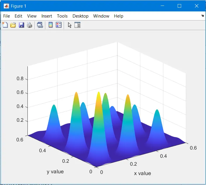
RESULTS FOR GLOBAL MAXIMA
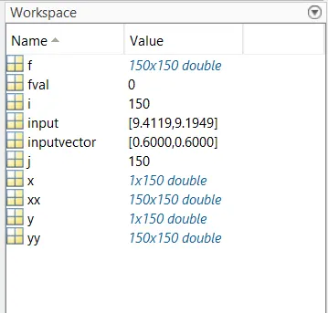
EXPLANATION OF THE CODE
- Firstly starting the program with ‘close all ‘, ‘clear all’ and clc are used to close previous plots and clear the workspace and command window respectively.
- Then we use the linspace command to specify the range for both inputs for and y from 0 to 0.6 with 150 values between them.
- Now, we use the mesh grid command to convert one dimensional array into 2- dimensional array. These 2 dimensional array are named as ‘xx’ and ‘yy’ in the code.
- We use the ‘for loop’ to calculate the stalagmite function, in which I and j is assigned as each value of ‘x’ and ‘y’ of the 2- dimensional array.
- Now for each value of x and y an array is created named as input and this input
Will be a row vector (which is two column matrix)
- The first column of the input vector is defined as values of ‘xx’ and the second column of the input vector is defined as ‘yy’ matrix values.
- Now, using these values the stalagmite function is calculated. the function for the stalagmite is written below :
function[f]=stalagmite(input vector)
x=inputvector(1);
y=inputvector(2);
f1=(sin(5.1*pi*x+0.5))^6;
f2=(sin(5.1*pi*y+0.5))^6;
f3=exp(-4*log(2)*(x-0.0667)^2/0.64);
f4=exp(-4*log(2)*(y-0.0667)^2/0.64);
f=(f1*f2*f3*f4);
end
- Now, this above function stalagmite takes the input vector and calculates the value for ‘f ‘.
- Then the two ‘for loops ‘generates the data for the plot which we need to generate a stalagmite graph.
- Surface command creates a primitive, three-dimensional surface The function plots the values in matrix Z as heights above a grid in the x-y plane defined by X and Y (Z). [ if the command entered as ‘surface (x,y,z)’]
- The ‘shading ‘interp ‘command is used to remove the grids that formed on the grid which gives us a better and smooth looking plot.
- To optimize the function we use an in built command which is ‘ga’, then this command performs genetic algorithm on the function which is defined and gives us outputs as optimized results.
PLOTTING GLOBAL MINMA AND FINDING THE MINIMUM OF THE FUNCTION
clear all
close all
clc
x=linspace(0,0.6,150);
y=linspace(0,0.6,150);
numcases=50;
%creating a 2dimensional mesh
[xx yy]=meshgrid(x,y);
tic
%evaluating the stalgamite function
for i=1:length(xx)
for j=1:length(yy)
%to get x and y values
inputvector(1)=xx(i,j);
inputvector(2)=yy(i,j);
%function definition
f(i,j)=stalagmite(inputvector);
end
end
%study 1 - statistical behaviour
for i= 1:numcases
[input, fopt(i)] = ga(@stalagmite,2);
xa(i)=input(1);
ya(i)=input(2);
end
time=toc;
%plotting1
figure(1)
subplot(2,1,1)
hold on
surf(x,y,f)
shading interp
plot3(xa,ya,fopt,'marker','o','markersize',5,'markerfacecolor','g')
title ('Unbounded inputs')
subplot(2,1,2)
plot(fopt)
xlabel('Iterations')
ylabel('function minimum')
function[f]=stalagmite(inputvector)
x=inputvector(1);
y=inputvector(2);
f1=(sin(5.1*pi*x+0.5))^6;
f2=(sin(5.1*pi*y+0.5))^6;
f3=exp(-4*log(2)*(x-0.0667)^2/0.64);
f4=exp(-4*log(2)*(y-0.0667)^2/0.64);
f= - (f1*f2*f3*f4);
end
FOR FINDING THE MINIMUM FUNCTION BY GA
PLOT FOR UNBOUNDED INPUTS
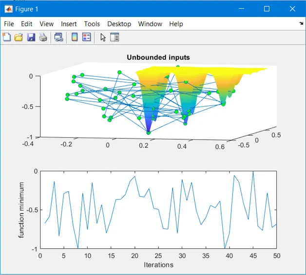
RESULTS FOR STUDY 1
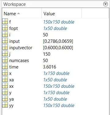
EXPLANATION OF THE CODE
- The above study shows us the statistical behaviour of genetic algorithm in matlab.
- The code similar to finding the global maxima only change is that we are performing ga for some number of iteration and observe all the values are changing for each iteration.
- In this case since we are finding out the global minima , the function for the stalagmite will be :
function[f]=stalagmite(input vector)
x=inputvector(1);
y=inputvector(2);
f1=(sin(5.1*pi*x+0.5))^6;
f2=(sin(5.1*pi*y+0.5))^6;
f3=exp(-4*log(2)*(x-0.0667)^2/0.64);
f4=exp(-4*log(2)*(y-0.0667)^2/0.64);
f= - (f1*f2*f3*f4);
end
- Now x and y values are being defined and then we define the number of times ga has to be performed as a variable num cases and have given it a value.
- Now, we use the mesh grid command to convert one dimensional array into 2- dimensional array. These 2 dimensional array are named as ‘xx’ and ‘yy’ in the code.
- We use the ‘for loop’ to calculate the stalagmite function, in which i and j is assigned as each value of ‘x’ and ‘y’ of the 2- dimensional array.
- Then we declare the number of iteration as 50 into numcases.
- We run for loop for num cases to implement genetic algorithm .
- For the first case study we are just calling the function ga, storing the values of x and y and also the optimum value the function predicts.
- The optimum value at each iteration and its corresponding input is stored in a row vector into input and fopt. The input variable is further broken down into xa and ya variables.
- The tic- toc command is used to measure and record the time taken by the ga function to finish 50 iteration.
- Subplot function divides the figure 1 into 2 rows
- The first row contains inverted stalagmite plot which is created by the in - built surf function by passing x and y and corresponding stalagmite output value f.
- The 3D plot of different optimum values as predicted by ga functions over 50 iterations. The 3D plot of optimum values and corresponding inputs achieved by plot 3
- The second row contains a simple 2D plot which depicts optimum value over different iterations. In built plot function plots array element along y – axis against their index along x – axis.
STUDY 2
clear all
close all
clc
x=linspace(0,0.6,150);
y=linspace(0,0.6,150);
numcases=50;
%creating a 2dimensional mesh
[xx yy]=meshgrid(x,y);
tic
%evaluating the stalgamite function
for i=1:length(xx)
for j=1:length(yy)
%to get x and y values
inputvector(1)=xx(i,j);
inputvector(2)=yy(i,j);
%function definition
f(i,j)=stalagmite(inputvector);
end
end
tic
%study 2 - statistical behaviour - with upper and lower bounds
for i= 1:numcases
[input, fopt(i)] = ga(@stalagmite,2,[],[],[],[],[0;0],[1;1]);
xa(i)=input(1);
ya(i)=input(2);
end
time=toc;
%plotting
figure(2)
subplot(2,1,1)
hold on
surf(x,y,f)
shading interp
plot3(xa,ya,fopt,'marker','o','markersize',5,'markerfacecolor','g')
title ('bounded inputs')
subplot(2,1,2)
plot(fopt)
xlabel('Iterations')
ylabel('function minimum')
function[f]=stalagmite(inputvector)
x=inputvector(1);
y=inputvector(2);
f1=(sin(5.1*pi*x+0.5))^6;
f2=(sin(5.1*pi*y+0.5))^6;
f3=exp(-4*log(2)*(x-0.0667)^2/0.64);
f4=exp(-4*log(2)*(y-0.0667)^2/0.64);
f=-(f1*f2*f3*f4);
end
PLOT FOR BOUNDED INPUTS
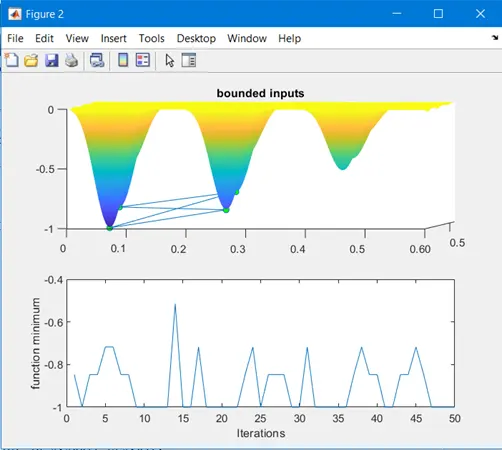
RESULTS FOR STUDY 2
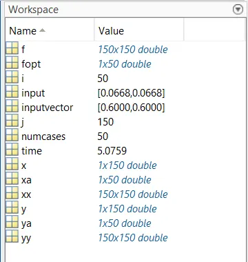
EXPLANATION OF THE CODE
- In case for the second study, in addition to the above code here we are specifying the upper and lower limits of inputs x and y, lower and upper limit of both x and y are set as 0 and 1 respectively.
- The above program also uses the same input and function output.
- The same tic- toc command is used to measure and record the time taken by the ga function to finish 50 iteration.
- In this case also the ga is running for 50 iterations but with specified limits restricting the values of both inputs x and y between 0 and 1. They are specified in row vector format as [0, 0] and [1,1] as upper and lower limit respectively .
- As in the first case the optimal and the corresponding inputs are stored in input and fopt variables.
- 3D and 2D plots are plotted and is printed into the console.
STUDY 3
clear all
close all
clc
x=linspace(0,0.6,150);
y=linspace(0,0.6,150);
numcases=50;
%creating a 2dimensional mesh
[xx yy]=meshgrid(x,y);
tic
%evaluating the stalgamite function
for i=1:length(xx)
for j=1:length(yy)
%to get x and y values
inputvector(1)=xx(i,j);
inputvector(2)=yy(i,j);
%function definition
f(i,j)=stalagmite(inputvector);
end
end
%study 3 - increasing ga iterations
options=optimoptions('ga');
options=optimoptions(options,'populationsize',170);
tic
for i= 1:numcases
[input, fopt(i)] = ga(@stalagmite,2,[],[],[],[],[0;0],[1;1],[],[],options);
xa(i)=input(1);
ya(i)=input(2);
end
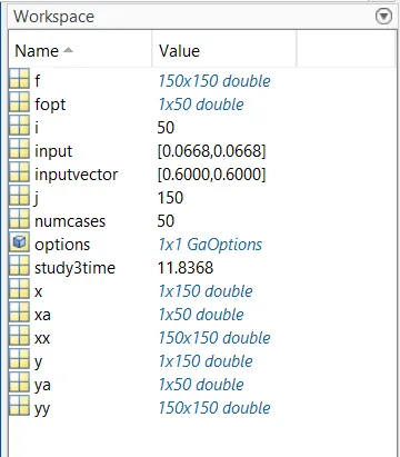
study3time=toc
%plotting
figure(3)
subplot(2,1,1)
hold on
surf(x,y,f)
shading interp
plot3(xa,ya,fopt,'marker','o','markersize',5,'markerfacecolor','g')
title ('bounded inputs with modified population size')
subplot(2,1,2)
plot(fopt)
xlabel('Iterations')
ylabel('function minimum')
function[f]=stalagmite(inputvector)
x=inputvector(1);
y=inputvector(2);
f1=(sin(5.1*pi*x+0.5))^6;
f2=(sin(5.1*pi*y+0.5))^6;
f3=exp(-4*log(2)*(x-0.0667)^2/0.64);
f4=exp(-4*log(2)*(y-0.0667)^2/0.64);
f=-(f1*f2*f3*f4);
end
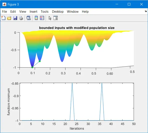
PLOT FOR BOUNDED INPUTS WITH HIGHER POPULATION
RESULTS FOR STUDY 3
EXPLANATION OF THE CODE
- In the above program we specify the initial population in which an option object for ga function, a part of the optimization toolbox by using optimoptions function by mentioning ga as a parameter. This creates an option instance for ‘ga’
- The population size is increased to 170.
- For each iteration the option instance is passed to the ga function as per the syntax.
- Similarly in the last two cases, the time is recorded for study 3, since the initial population was increased, it takes lot of time for each iteration .
- The two graphs showing stalagmite function, fopt and input and 2D graph are plotted.
ERRORS
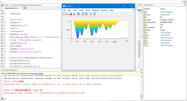
- When I used the plot command it resulted in an error, to rectify this mistake I used the plot3 command (to plot 3 axes) which resulted in the proper graph.
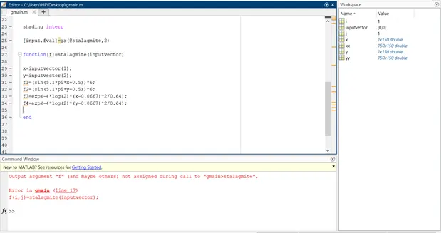
- b) When I did not mention the output ‘f ’ for the function it resulted in an error , to correct this error I mentioned the function
F= (f1. F2. F3. F4)
REFERENCES
https://in.mathworks.com/help/gads/ga.html
https://in.mathworks.com/discovery/genetic-algorithm.html
CONCLUSION
It can be said that more the number of iteration better will be the convergence of getting the minimum value irrespective of how much we run ‘ga’