Final Project: Electric Rickshaw modelling

AIM:

Create a detailed MATLAB model of an electric rickshaw (three-wheel passenger vehicle) as per details below:

Rear wheels driven by PM brushed type motor

Assume efficiency points of motor controller and motor

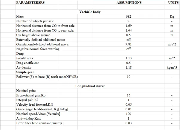
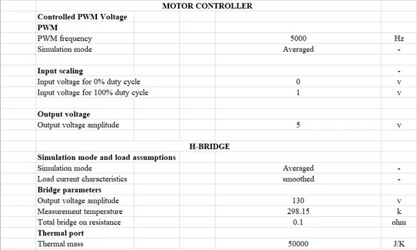
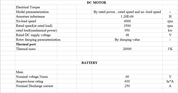
Make an excel sheet of all input and assumed data

Results: For any three standard driving cycles show energy consumption, temperature rise of motor and controller for 100 km constant speed driving at 45Kmph

(Note- The Simulink model file should be compulsorily attached)

1. Create a detailed MATLAB model of an electric rickshaw (three-wheel passenger vehicle) as per details below:

Rear wheels driven by PM brushed type motor

Assume efficiency points of motor controller and motor

Make an excel sheet of all input and assumed data

Results: For any three standard driving cycles show energy consumption, temperature rise of motor and controller for 100 km constant speed driving at 45Kmph

(Note- The Simulink model file should be compulsorily attached)

ELECTRIC RICKSHAW

In today’s world electric rickshaw have become popular among Indian drivers and commuters. Electric rickshaw is eco-friendly battery operated three wheelers which have better economy and lower maintenance cost because of which these electric rickshaws are in high demand. During operation electric rickshaws does not emit toxic pollutants in the air. Electric rickshaws in India are light in weight so as to prolong the life and performance of the battery. The electronic components that constitute the powertrain are motor, controller, harness, batteries and throttle. Any mismatch of these components is undesirable and may compromise vehicle performance.

Chassis is the important part which ensures safety of the vehicle which is made up of mild steel. The chassis is manufactured by a professional electric rickshaw manufacturer is robust as the design is applicable to all technical parameters. The chassis if not manufactured correctly will lead to problems in handling and could be easily damaged. Proper treatment should be carried out to the metal surface so that corrosion does not take place. Lesser the weight better will be the efficiency, materials that are used are fibre- reinforced plastic, aluminum, composite materials and low-density metals. Fibre – reinforced material is a very good alternative as it is very strong, highly durable, cheap, non- conducting, can withstand weather and can be easily repaired in case of damage. The body is attached to chassis by bolts and in some cases, it is welded also. The body is built in such a way keeping in mind the quality and design which is aerodynamic and ensures safety of the driver. High quality couplers should be required to ensure proper connection and also should be insulated to prevent water and moisture. High quality electrical components should be used as this will lower resistance and heat losses and will increase the efficiency.

The motor power used in most electric rickshaws is of the range 650-1250W, the government norms is 650W. If higher watts are used it will adversely affect the battery life. The controller used is 40A and 48V output. 14,18 and 24 MOSFETS are used and powers all electric components. A quality controller should be used to increase the performance of the motor and overheating problems.

Braking plays an important role as improper functioning of the brakes may heat up the motor and controller and may damage the brake shoes and it may also reduce the mileage of the vehicle.

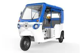
SCHEMATIC DIAGRAM OF AN ELECTRIC RICKSHAW

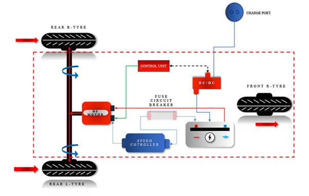
Electric rickshaw works on the same principle as electric vehicle. They run on lithium-ion battery pack. The motors used are DC motors. Mostly electric rickshaws are rear wheel driven. The power from the battery pack goes through an AC charger circuit with a rectifier so as to convert them to DC power. After the battery pack is charged, the signals are sent to the electronic control unit. The main purpose of the electronic control unit is to control the speed according to the drivers input (accelerator and brake). These pulses are then sent to the DC motor which transfers power to the wheels.

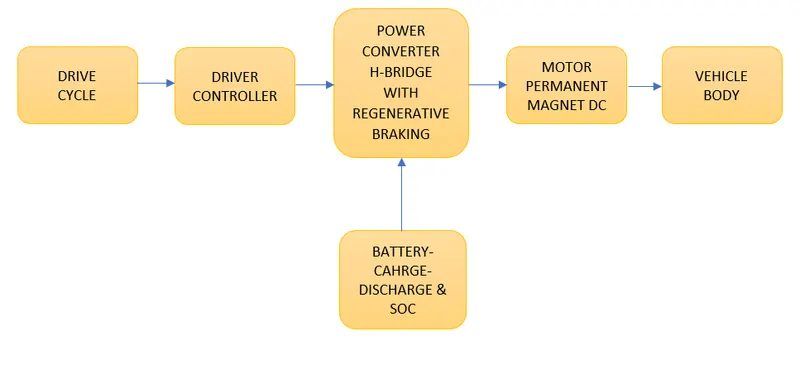
BLOCK DIAGRAM

VEHICLE BODY SUBSYSTEM

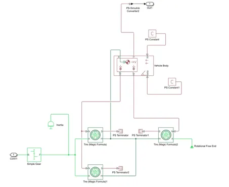
The following blocks that were used for the creation of the model are:

• Tire (magic formula)
• Vehicle body
• Simple gear
• Inertia
• PS- Simulink converter
• Rotational free end

• TIRE (MAGIC FORMULA)

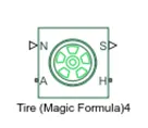
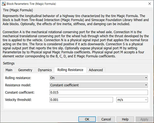
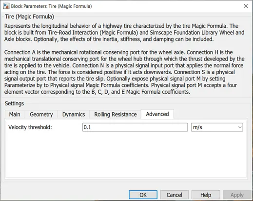
The magic tire block models a tire with longitudinal behaviour which is given by a magic formula an empirical equation based on four fitting coefficients. Under constant or variable pavement conditions this block can model tire dynamics. The longitudinal direction of the tire is same as the direction of motion as it rolls on the pavement.

Connection A is referred to the mechanical rotational conserving port for the wheel axle. Connection H is the mechanical translational conserving port for the wheel hub through which the thrust is developed by the tire which is applied to the wheel. Connection N is a physical signal input port that applies the normal force acting on the tire. If it is acting downwards the force is considered positive. Connection S is a physical signal output port reveals the tire slip.

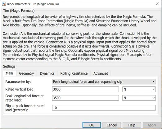
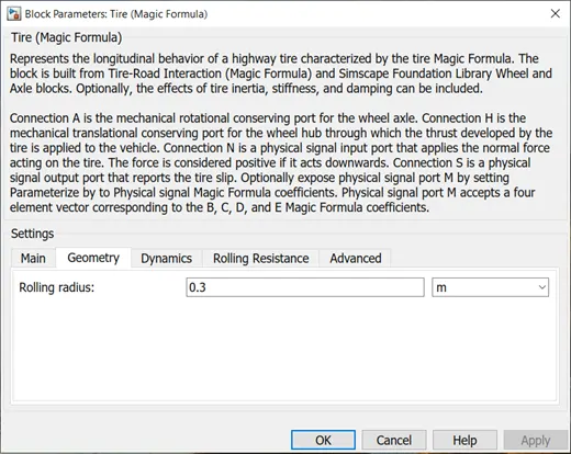
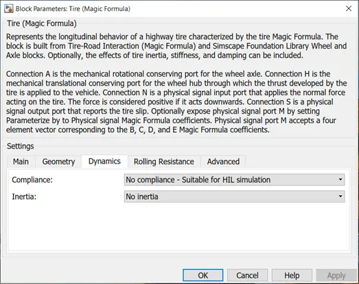
• VEHICLE BODY

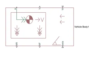
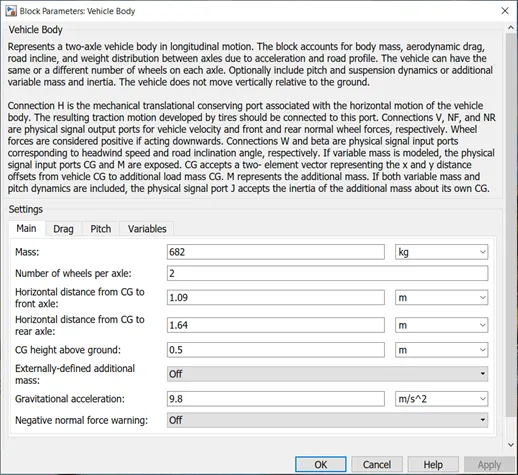
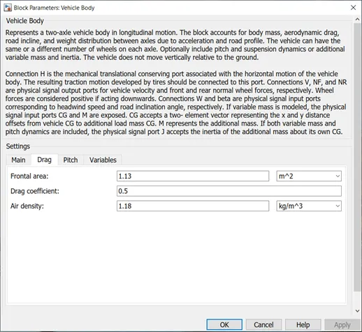
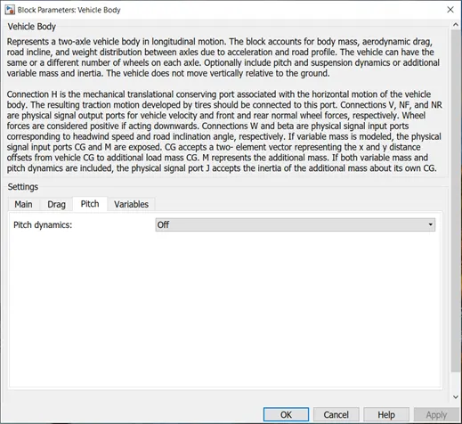
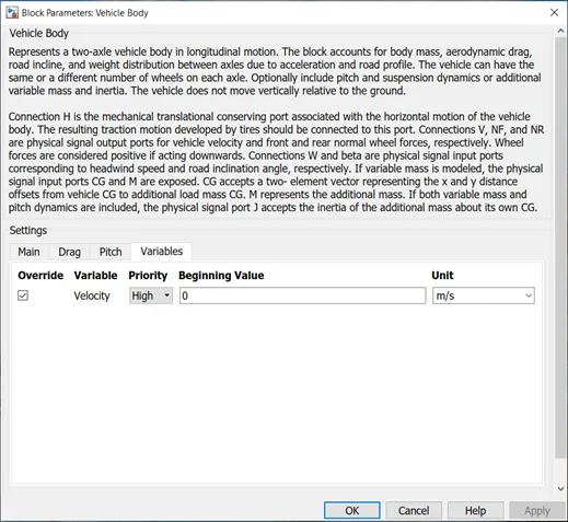
This vehicle body block is a representation of a two – axle vehicle body in longitudinal motion. The vehicle can have the same or different number of wheels on each axle. The vehicle can have a centre of gravity that is at or below the plane of travel. This block accounts for body mass, aerodynamic drag, road incline and weight distribution between axles due to acceleration and road profile which optionally includes pitch and suspension dynamics. The vehicle does not move vertically relative to the ground.

Connection H is the mechanical translational conserving port which is associated with the horizontal motion of the vehicle body. The traction motion developed by the tires should be connected to this port.

Connections V, NF and NR are physical signal output ports that represents vehicle velocity and front and rear normal wheel forces. These wheel forces are considered positive if acting downward. Connections W and beta are physical signal ports that signify headwind speed and road inclination angle respectively.

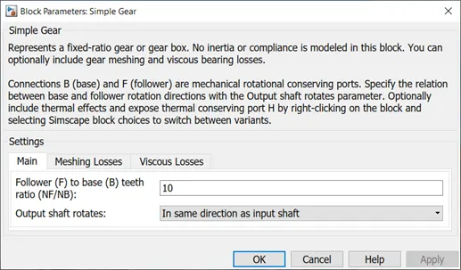
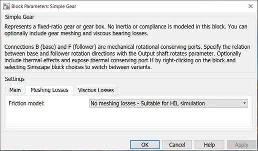
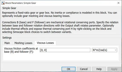
• SIMPLE GEAR

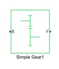
The simple gear box represents the gearbox that constrains the connected driveline axes of the base gear B and the follower gear F to corotate with a fixed ratio that is specified. Connections B which is the base and F the follower are mechanical rotational conserving ports.

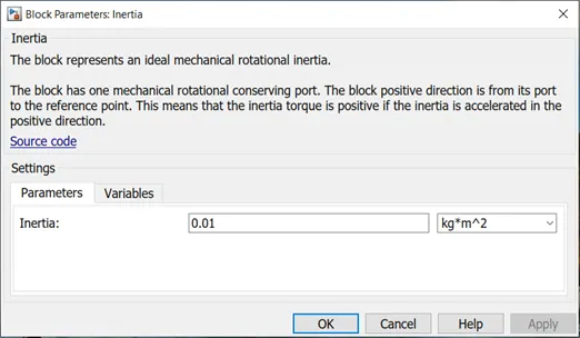
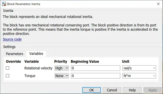
• INERTIA

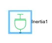
This block represents a mechanical rotational inertia and is given by the following equation :

T=J dω

dt

where,

T= inertia torque

J = inertia

ω = angular velocity

t = time

• PS-SIMULINK CONVERETER

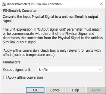
The PS – Simulink converter block converts a physical signal into Simulink.

• ROTATIONAL FREE END

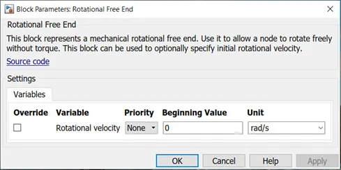
This block represents a mechanical rotational port that rotates freely without torque.

EXPLANATION OF VEHICLE BODY SUBSYSTEM

• Transmission is an important aspect of the electric rickshaw which is used to supply the propulsion power from the motor and then the wheels.
• For the creation of the above subsystem the following blocks that were used were Tire (Magic formula) block, simple gear block, vehicle body, inertia and ps- Simulink converter so as to create the base for the model.
• Firstly, the wheels of the vehicle are modelled by using the Tire block. Three tire blocks are created for the vehicle and named them as front and rear wheels.
• For the tire block there are various parameters which can be edited according to the requirement. During the simulation default parameters of the tire block were used.
• Then all the ports of each tire block are connected with each other. Port A represents axle so the rear wheels A ports are connected with each other which signifies that they are on the same axle. The front wheel A port is connected to a rotational free end.
• Then the H port represents the hub and all the H ports are connected to each other.
• The N and S port represents the normal force and slip of the tire respectively. So, the normal force on the rear wheels is the same, so the N port of both rear wheels is connected with each other and similarly for the front wheel normal force. The port S represents the slip occurring in the wheel. The port can be connected or can be ignored. In the above model it is connected to a PS Terminator block which terminates the physical signal outputs.
• Then a vehicle body diagram is used which represents the vehicle dynamics where there are various parameters which can be changed according to the requirement.
• The NR and NF port in the vehicle body represents the normal force on rear and front tires respectively. So, the N port of the front and rear tires are connected with NR and NF ports accordingly.
• The H port in the vehicle body is associated with the horizontal motion of the body and is connected to the H port of all the tires.
• The W and BETA port represents the wind speed and road inclination angle which can be entered as an input. In the above model the W and the BETA port are connected to a PS constant block since we have assumed both to be zero.
• The port V in the vehicle body represents the velocity output from the electric rickshaw. So, this is connected to the output port. Since the power from the motor has to be transmitted to the wheels a transmission block is used which is a SIMPLE GEAR BLOCK. This block is connected to the rear wheel axle since the model is considered as a rear wheel drive.
• Finally, the subsystem is modelled where the input of the system is the power given to the simple gear box and output is the velocity of the electric rickshaw.

MOTOR CONTROLLER SUBSYSTEM MODEL (WITH TEMPERATURE SENSOR)

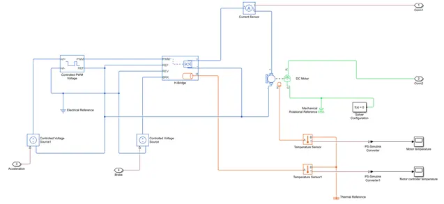
The following blocks that were used for the creation of the model are:

• Controlled voltage source
• Controlled PWM voltage
• H-Bridge
• Current sensor
• Solver configuration
• DC motor
• Mechanical rotational reference
• Temperature sensor
• Thermal reference
• Electrical reference
• Scope

• CONTROLLED VOLTAGE SOURCE

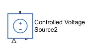
The controlled voltage source depicts an ideal voltage source which is powerful enough to maintain the specified voltage at its output irrespective of the current flowing through the source.

The output voltage V = V_s, where V_{s is} the numerical value presented at the physical signal port.

• CONTROLLED PWM VOLTAGE

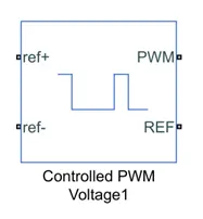
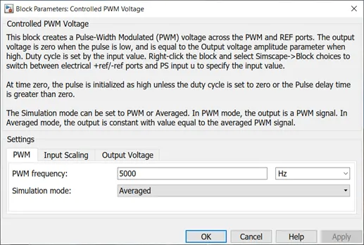
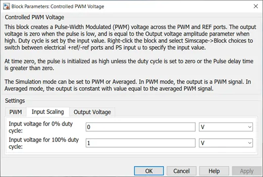
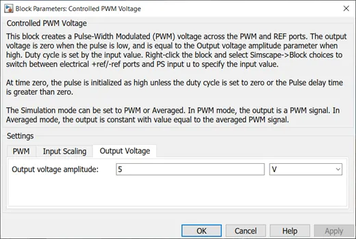
The Controlled PWM voltage block represents a pulse width modulated (PWM) voltage source. This block has two modelling variants by right clicking on the block and then selecting simscape and then block choices which are electrical input ports and PS input

• Electrical input ports
• Ps input

• ELECTRICAL INPUT PORTS

This block calculates the duty cycle which is based on the reference voltage across ref+ and ref- ports. This modelling variant is default.

• PS INPUT

Specifies the duty cycle value directly by using an input signal port.

For electrical inputs ports variant of the block, the duty cycle calculated is :

100*V_ref – V_min / V_max - V _min %

Where,

V_ref is the reference voltage across ref+ and ref- ports

V_min is the minimum reference voltage

V_max is the maximum reference voltage

• H-BRIDGE

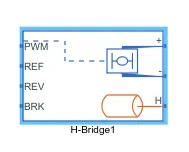
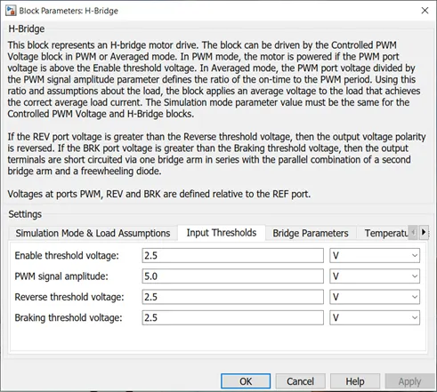
H- bridge block output is a controlled voltage that depends on the input signal at the PWM port. The H- bridge is connected to Pulse Width Modulation for controlling of the voltage signals and the output of the H bridge is connected to the terminals to provide the controlled voltage to the D.C motor.

The ports in H- BRIDGE are:

• PWM – this stand for pulse width modulation which provides the voltage pulses to H- bridge either in PWM or average mode.
• REF - is the floating zero-volt reference.
• REV - Voltage that controls when to reverse the polarity of the H- bridge block output.

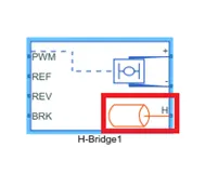
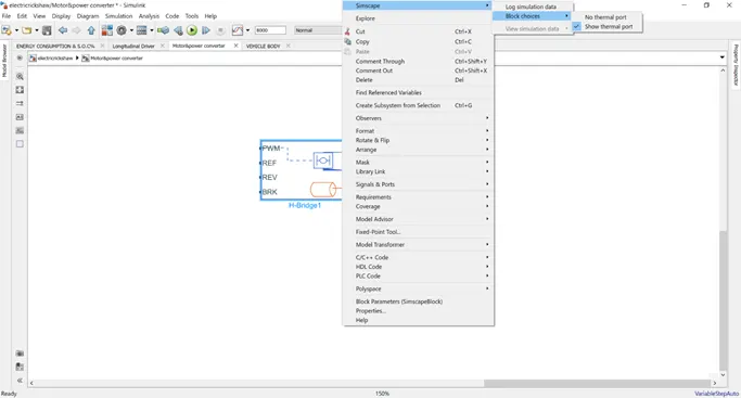
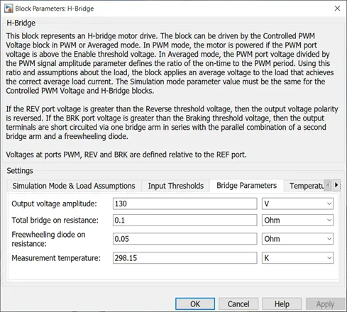
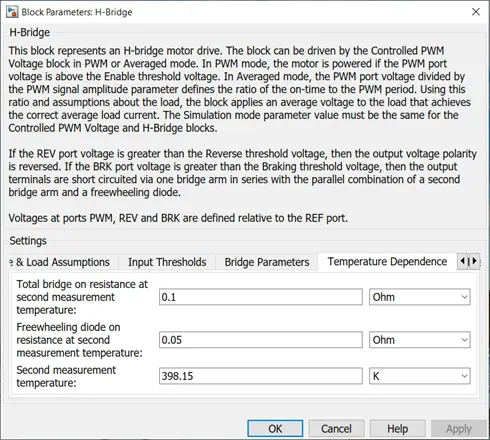
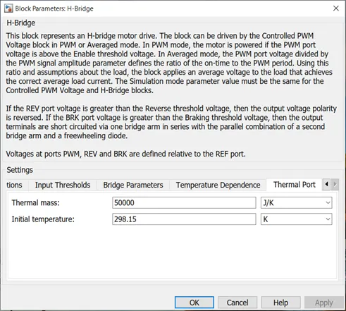
In this block the thermal port is also added which is the H port so as to measure the temperature of the motor controller. This port is added by right clicking on the block and then selecting simscape option block choices and there will be 2 options of no thermal port and show thermal port as shown below:

• CURRENT SENSOR

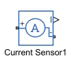
The current sensor block represents an ideal current sensor. It is a device that converts current measured in any electrical branch into physical signal proportional to the current. The connection + and – in the block are electrical conserving ports through which the sensor is inserted in the circuit.

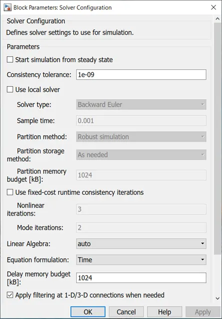
• SOLVER CONFIGURATION

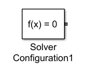
The solver configuration block requires solver settings information for simulation. The block specifies the solver parameters that the model requires before running the simulation.

• D.C MOTOR

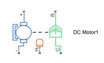
There are 2 sides to the block as seen above the mechanical side and electrical side. The mechanical side has 2 ports, C and R. The C refers to casing and R for the rotation of the rotor. The electrical side has a positive and negative terminal for the voltage to be applied. The C port of the mechanical side needs to be connected to a mechanical rotational reference because it will be stationary. The R port will be connected to the simple gear of the vehicle body block.

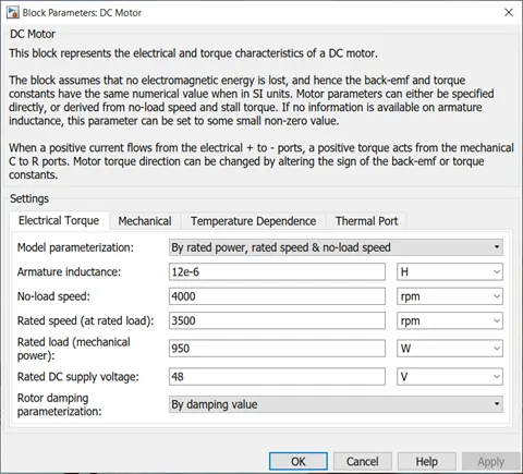
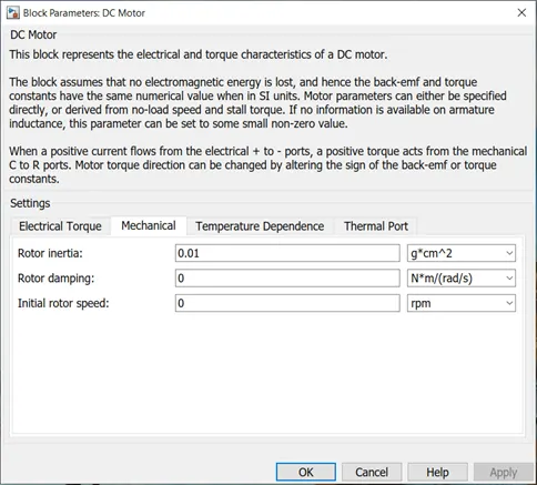
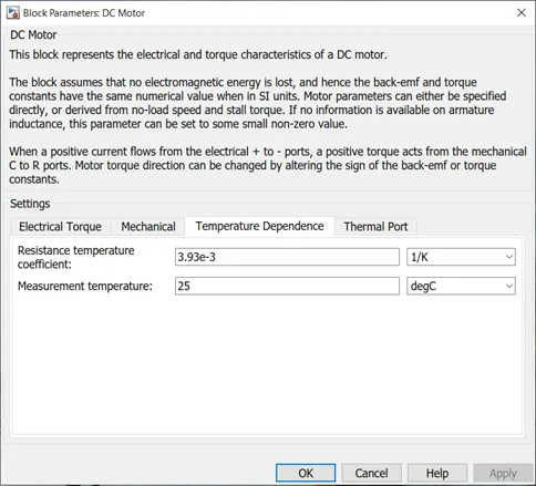
D.C motor block represents the torque and electrical characteristics of D.C motor using the equivalent circuit model.

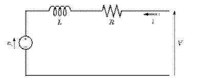
The resistor R refers to the resistance which is specified in the armature resistance parameter. The inductor corresponds to the inductance which is specified in the armature inductance parameter.

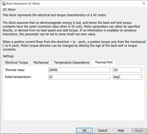
Similarly, just as for the motor controller H-PORT is added, even for the motor H-PORT is added so as to measure the temperature of the motor by right clicking on the block and go to simscape option block choices and there will be 2 options of no thermal port and show thermal port.

• MECHANICAL ROTATIONAL REFERNCE

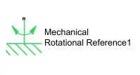
The mechanical rotational reference block represents a reference point or frame for all mechanical ports.

• TEMPERATURE SENSOR

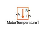
This block represents the temperature sensor, a device that determines the temperature differential measured between two points without drawing any heat.

A and B are thermal conserving ports are connected to two points where the temperature is being monitored. T port is a physical signal port that gives the output of the temperature differential value.

The block positive direction is from port A to port B. The temperature measured between two ports are T=T_A – T_B

The block has the following ports:

• A – thermal conserving port is with the sensor positive probe.
• B – Thermal conserving port is with the sensor negative probe.
• T – physical signal output port for temperature.

• THERMAL REFERNCE

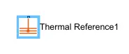
This block represents a thermal reference point, a point with an absolute zero temperature with respect to all the temperatures in the system are determined.

• ELECTRICAL REFERENCE

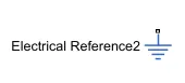
The electrical reference ground represents an electrical ground. Electrical conserving ports of all the blocks that are directly connected to the ground must be connected to an electrical reference block.

• SCOPE

Scope is used for viewing the graph of the signals after the simulation is run.

EXPLANATION OF THE MOTOR CONTROLLER SUBSYSTEM

• The motor controller subsystem contains mainly of H- bridge and a controlled PWM voltage block and D.C motor
• A controller is needed to control the motor according to the needs which is why a controller block is used which is the H-bridge
• H- bridge is used to supply power from the battery to the D.C motor. H- bridges has four switches that give the controlled D.C voltage supply to the D.C motor that can control the supply of voltage.
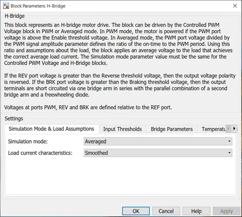
• In H-bridge block parameters there are two options for simulation mode to chooses from either averaged or PWM but averaged mode is chosen since the simulation time is in mins or hours and it is faster as compared to PWM mode.
• In the H-BRIDGE BLOCK there is a PWM signal input port, where PWM input can be given to this port. The REF and REV ports are grounded using electrical reference block. This is done to prevent reverse operation of the motor. BRK port is connected to a controlled voltage source which helps in carrying out regenerative braking.
• In the H-BRIDGE BLOCK there is a thermal port added which is connected to a temperature sensor and then to a scope through a PS-SIMULINK converter so as to measure the temperature of the motor controller.
• PWM signals is given to the H- BRIDGE BLOCK by using CONTROLLED VOLTAGE BLOCK. This block helps in creating PWM signals which are generated according to the variable voltage.
• The PWM and REF port of the controlled PWM voltage is connected to PWM and REF port of the H- BRIDGE. The ref- port is grounded since we don’t need negative voltage and is connected to the REF and REV port of the H-BRIDGE. The ref+ port is connected to CONTROLLED VOLTAGE BLOCK so that the input voltage is the same always.
• Controlled PWM voltage block is connected to the input PWM port in the H- bridge block.
• This block will apply pulses and based on these pulses from the fixed battery voltage variable output voltage will be available to the motor and the motor torque and motor speed are changed.
• Now an appropriate motor is selected for the electric rickshaw so a C motor block is used to represent the DC motor. In the D.C motor block the parameters were changed like the rated D.C voltage of the motor, rated load, no load speed, rated speed according to the rickshaw needs.
• The motor block has 4 ports -, +, C and R where – and + ports are the motor terminals where the power supply is connected and the positive torque is from port C to R, and port C is considered as fixed end of motor so it is connected to the mechanical rotational reference block to which a solver configuration block is added. The + port of the DC motor is connected to the H-BRIDGE through current sensor and the negative port of the DC motor is connected to negative of the H-BRIDGE as well as the REF port of the H- BRIDGE.
• The port R is connected to vehicle dynamics subsystem input which is the simple gear box. Similary just as in case of H-BRIDGE a thermal port is also added to the DC motor so as to measure the temperature of the motor.
• Finally, the subsystem is created with the following blocks and the subsystem will control the power supply to the D.C motor.

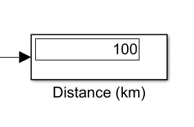
DISTANCE CALCULATION

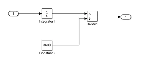
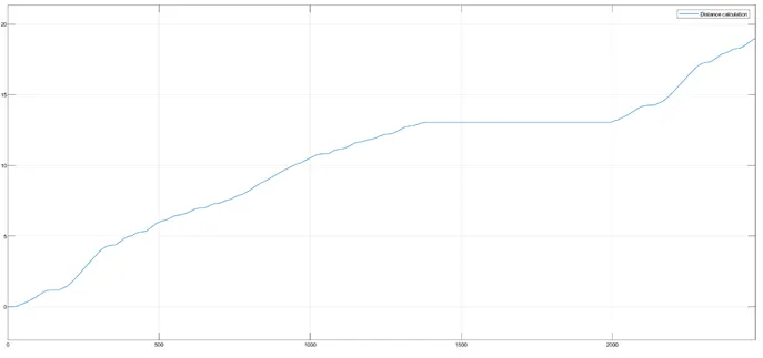
• In the above model for distance calculation the input is taken from the velocity feedback and it is integrated using the integrator block and divided by 3600.

ENERGY CONSUMPTION AND SOC%

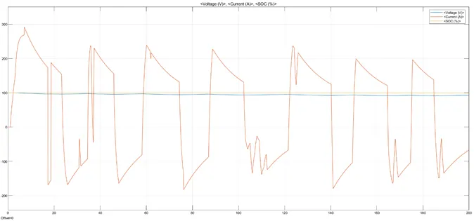
State of charge is defined as the measurement of available charge in the battery. When the battery is fully charged, it is considered to have 100% and when it is 0% it is said to be discharged. After the simulation is run, we get an estimate of the current and S.O.C of the battery with respect to time.

ENERGY CONSUMPTION AND SOC% SUBSYSTEM

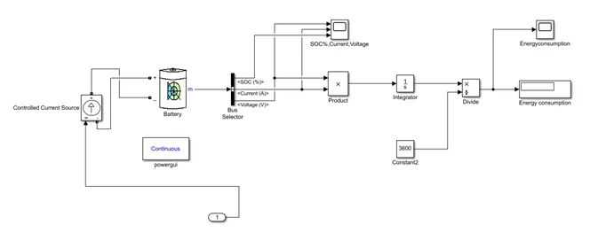
The following blocks that were used for the creation of the subsystem:

• Controlled current source
• Battery
• Bus selector
• Powergui
• Product
• Integrator
• Constant
• Product
• Divide
• Scope

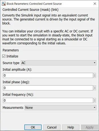
• CONTROLLED CURRENT SOURCE

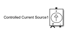
The controlled current source block converts the Simulink input signal into equivalent current source. The positive current direction is as shown by the arrow in the block icon.

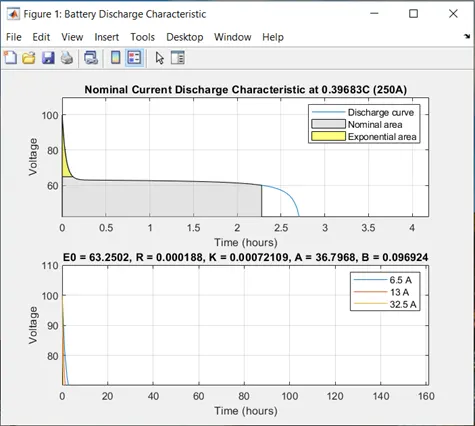
• BATTERY

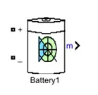
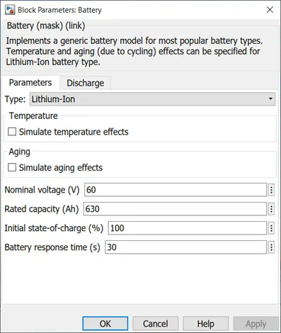
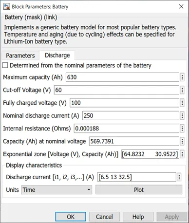
This block creates a generic dynamic model parameterized to represent most popular types of rechargeable batteries.

• BUS SELECTOR

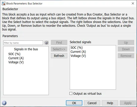
The output of the block specifies subset of elements of bus at its input. The block can output the specified elements as separate signals.

• POWERGUI

The power gui block chooses the following methods to solve the circuit:

• Continuous, which uses a variable step solver from Simulink
• Discretization of the electrical system for a solution at fixed time steps
• Phasor solution

This block is used for steady state and simulation results analysis and also for advanced parameter design. This block is required to simulate Simulink model that contain simscape electrical specialized power system blocks

EXPLANATION OF ENERGY CONSUMPTION AND SOC% SUBSYSTEM

• This subsystem consists of lithium -ion battery block, a controlled current source and a bus selector
• The current sensor is connected to the controlled current source through a PS Simulink converter where the + connection of the controlled source is connected to the negative port of the battery and the – connection is connected to the positive port of the battery.
• From the M port of the battery block we obtain the S.O.C, ampere and voltage values. These values are extracted using bus selector when it is connected to the m port.
• The ampere and the voltage output is connected to a product block and multiplied so as to get the energy consumption in watts.
• This output is then connected to an integrator block which will add those watts over the simulation time and gives the value in watt second.
• This watt second value is then converted to watt hour by dividing by 3600 to obtain the energy consumed by the electric rickshaw during the course of the simulation.

SIMULINK MODEL OF AN ELECTRIC RICKSHAW

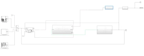
The following blocks that were used for the creation of the model:

• Drive cycle source (FTP75)
• Drive cycle source (wide open throttle)
• Drive cycle source (manual drive cycle)
• Multiport switch
• Longitudinal driver

• DRIVE CYCLE SOURCE

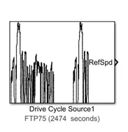
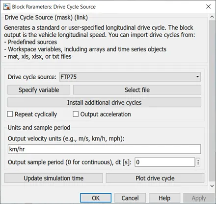
The Drive cycle source block generates a standard or user- specified longitudinal drive cycle. The output of this block is specified vehicle longitudinal speed.

This block predicts the engine torque and fuel consumption that a vehicle requires to achieve desired speed and acceleration for a given shift reference.

This block also studies and optimizes vehicle control, system performance and the system are good enough for multiple drive cycles.

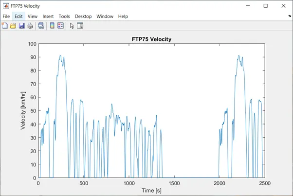
The plot of the drive cycle is shown below:

• DRIVE CYCLE SOURCE (WIDE OPEN THROTTLE)

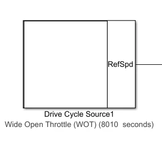
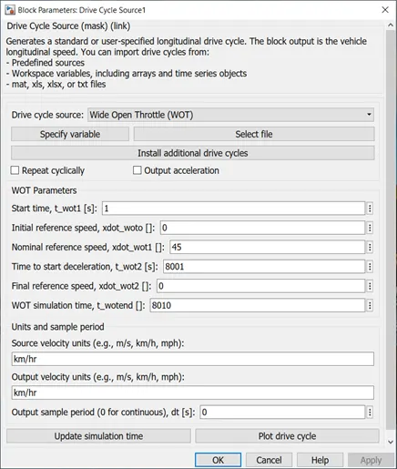
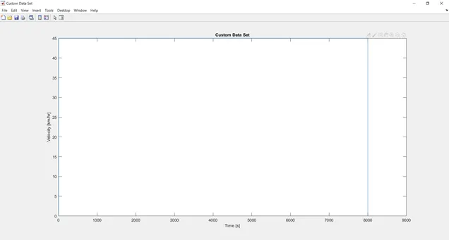
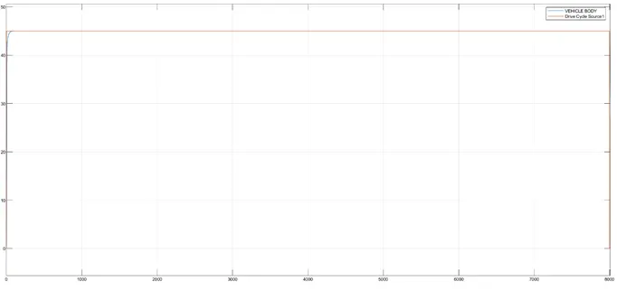
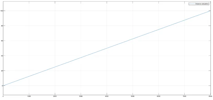
This is the wide-open throttle drive cycle in which the vehicle runs at a constant speed of 45 km/hr for a distance of 100km. So, the simulation time for this drive cycle is 8010 seconds.

Time= distance

speed

= 100 * 3600

45

= 8000 seconds

The plot of the drive cycle is shown below:

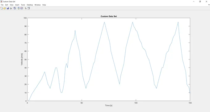
• DRIVE CYCLE SOURCE (CUSTOM DRIVE CYCLE)

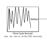
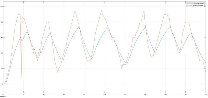
This is the custom-made drive cycle in excel sheet. The run time for this drive cycle is 200 seconds.

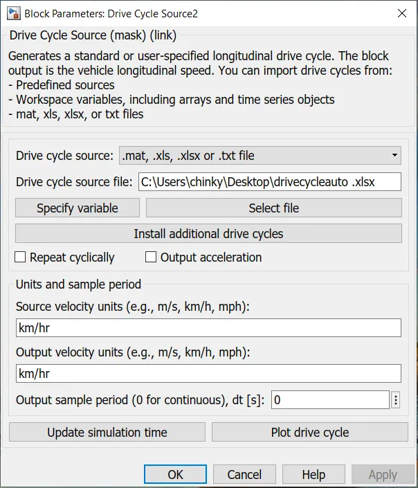
The plot of the drive cycle is shown below:

• MULTIPORT SWITCH

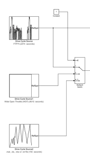
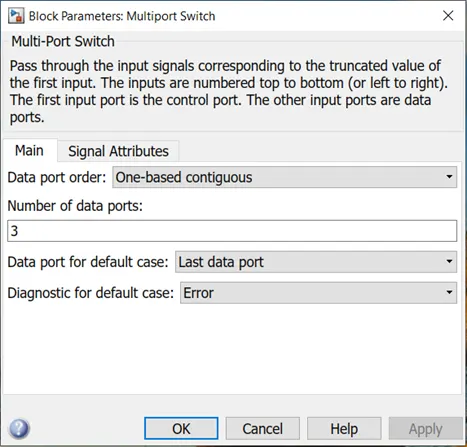
In the multiport switch block determines which of the several inputs to the block passes to the output. The block bases this decision on the value of the first input. The first input is the control input and the remaining inputs are the data points. To the control signal port, a constant block is added in which the position of which drive cycle should be connected.

• LONGITUDNAL DRIVER

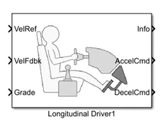
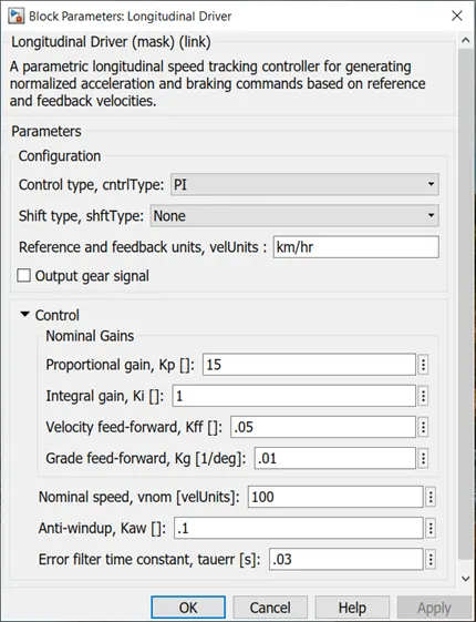
This longitudinal driver block uses a longitudinal speed – tracking controller. Based on feedback velocities and reference normalized acceleration and braking commands are generated which can vary from 0 through 1. This block is used to model the dynamic response of a driver.

EXPLANATION OF THE MODEL

• In the longitudinal driver block VelRef port is connected to a drive cycle and this drive cycle is compared with VelFdbk port where the vehicle speed is given as feedback. When the vehicle speed is more than the drive cycle speed, the block will out put it as deceleration which is DecelCmd port which is connected to one port of the controlled voltage source. If the speed of the vehicle is less than the drive cycle speed then the block will give output as acceleration which is AccelCmd port which is connected to controlled voltage source through a Simulink PS converter.
• The longitudinal driver block is connected to a standard drive cycle using drive cycle block through a multi-port switch
• In order to measure the speed of the electric rickshaw model, scope block is used where 2 input ports are made. One port takes the output velocity signal from the VEHICLE SUBSYSTEM BLOCK and another port takes the output signal from the drive cycle to the reference velocity port on the longitudinal driver block. This is done in order to show the plots of reference velocity and the actual velocity of the electric rickshaw and see how they compare with each other.
• The area under the velocity time graph depicts the distance travelled by the electric rickshaw. This means that integration is done with respect to time which gives the distance travelled. Integrator block is used to integrate the velocity signal that is the output from the subsystem. After the integrator block, divide block is used along with constant block with the value of 3600 in order to convert the integrated speed signal which is in kilometres per hour by 3600 which gives the distance travelled in kilometres.
• Finally, the electric rickshaw model is completed and once the simulation is run, we get the following results.

RESULTS:

• FOR FTP75 DRIVE CYCLE:

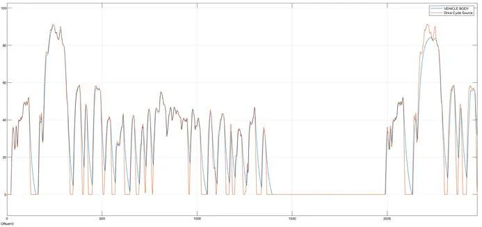
The scope below gives the input and output velocity graph. One is the drive cycle and other is the velocity feedback

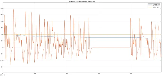
S.O.C %, VOLTAGE, CURRENT

Graph as shown below for FTP75 drive cycle which is run for 2474 seconds:

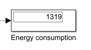
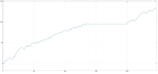
ENERGY CONSUMPTION

Graph as shown below for FTP75 drive cycle which is run for 2474 seconds:

MOTOR TEMPERATURE

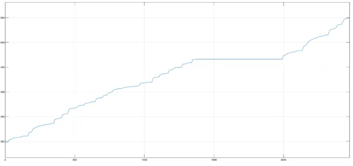
Graph as shown below for FTP75 drive cycle which is run for 2474 seconds which displays the value in degree K:

MOTOR CONTROLLER TEMPERATURE:

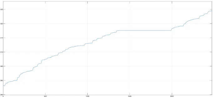
Graph as shown below for FTP75 drive cycle which is run for 2474 seconds which displays the value in degree K:

DISTANCE TRAVELLED:

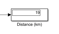
By running the electric rickshaw with FTP75 drive cycle for 2474 seconds. The distance travelled is 19Km

• DRIVE CYCLE SOURCE (WIDE OPEN THROTTLE)

The scope below gives the input and output velocity graph. One is the drive cycle and other is the velocity feedback

S.O.C %, VOLTAGE, CURRENT

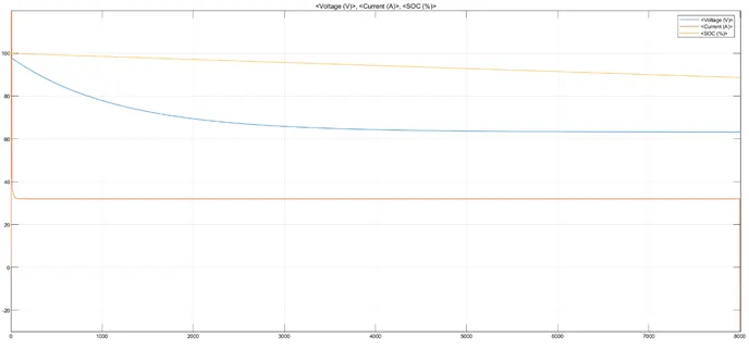
Graph as shown below for drive cycle (wide open throttle) which is run for 8010 seconds:

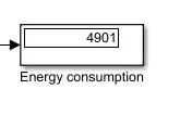
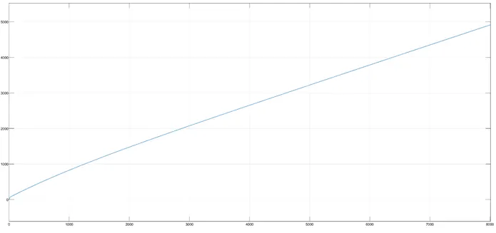
ENERGY CONSUMPTION

Graph as shown below for drive cycle (wide open throttle) which is run for 8010 seconds:

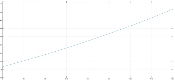
MOTOR TEMPERATURE

Graph as shown below for drive cycle (wide open throttle) which is run for 8010 seconds which displays the value in degree K:

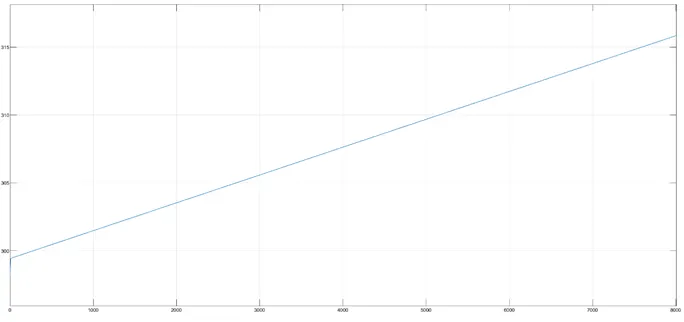
MOTOR CONTROLLER TEMPERATURE:

Graph as shown below for drive cycle (wide open throttle) which is run for 8010 seconds which displays the value in degree K:

DISTANCE TRAVELLED:

By running the electric rickshaw with drive cycle (wide open throttle) for 8010 seconds. The distance travelled is 100 km

• DRIVE CYCLE SOURCE (CUSTOM DRIVE CYCLE)

The scope below gives the input and output velocity graph. One is the drive cycle and other is the velocity feedback

S.O.C %, VOLTAGE, CURRENT

Graph as shown below for drive cycle (custom drive cycle) which is run for 200 seconds:

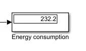
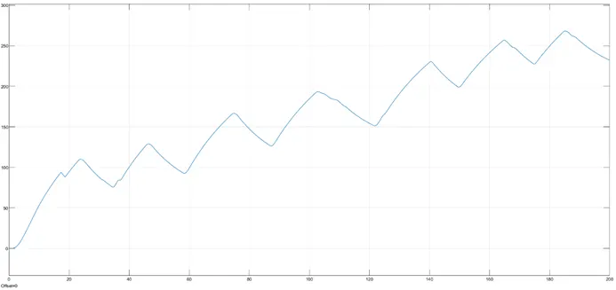
ENERGY CONSUMPTION

Graph as shown below for drive cycle (custom drive cycle) which is run for 200 seconds:

MOTOR TEMPERATURE

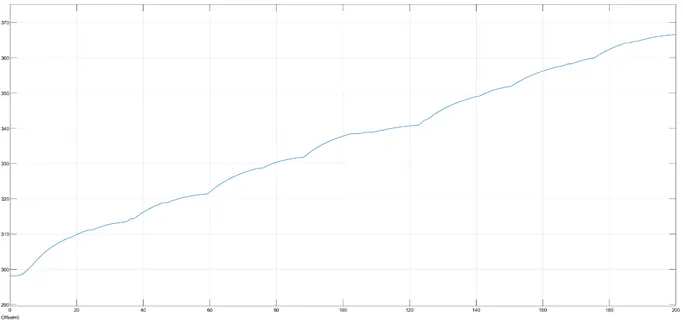
Graph as shown below for drive cycle (custom drive cycle) which is run for 200 seconds which displays the value in degree K:

MOTOR CONTROLLER TEMPERATURE:

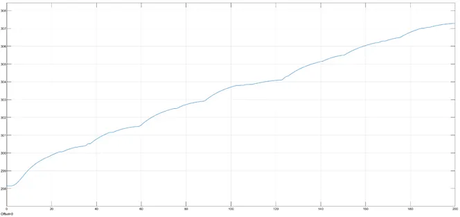
Graph as shown below for drive cycle (custom drive cycle) which is run for 200 seconds which displays the value in degree K:

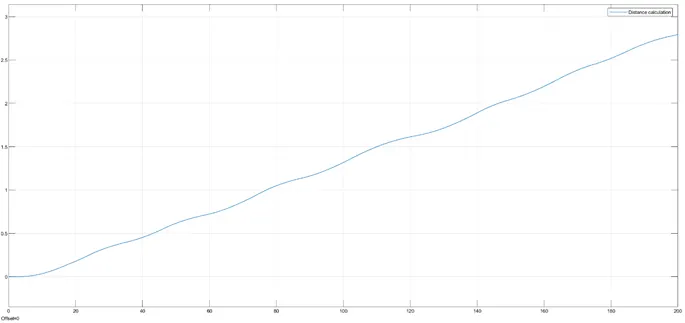
DISTANCE TRAVELLED:

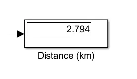
By running the electric rickshaw with drive cycle (custom drive cycle) for 200 seconds. The distance travelled is 2.794 Km

Drive Cycle	S.O.C%	Voltage (V)	Energy Cons (KWHR)	Motor Temp OK	Motor Controller Temp OK	Distance travelled (KM)
FTP75 (2474 seconds)	97.44	71.14	1319	549.7	324.5	19
Wide open throttle (8010 seconds)	88.64	63.34	4901	448.1	315.9	100
Custom drive cycle (200 seconds)	99.62	92.71	232	366.6	307.3	2.794

CONCLUSIONS:

Electric rickshaw was modelled with matalab using three different drive cycles. Cooling with liquid or air was not considered hence motor and motor controller temperature was high.