Week 3 - Solving second order ODEs

AIM:

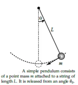
To describe the transient behaviour of a simple pendulum using mat lab, a second order ode is used which helps in determine the position of the bob at different times.

DESCRIPTION:

Ode is used to describe the transient behaviour of system, for example in case of simple pendulum. The motion of the pendulum depends upon newton’s second law of motion. The differential equation describes the position of the ball with respect to time.

This ode represents the equation of motion of a simple pendulum with damping:

D² θ /dt² + b/m dθ/dt + g/l sinθ =0

Let us assume θ = θ1

Then,

dθ/dt =dθ₁ /dt = θ₂

D² θ /dt² = D2 θ₁ /dt² = d/dt(dθ₁/dt ) = d/dt(θ₂)

D² θ /dt² + b/m dθ/dt + g/l sinθ =0

D² θ₁ /dt² + b/m dθ₁/dt + g/l sinθ₁ =0

D θ₂ /dt² + b/mθ₂ + g/l sinθ₁ =0

dθ₁/dt = θ₂ , dθ₂/dt = -b/m θ₂ - g/l sinθ₁

dθ/dt [θ₁ ; θ₂ ] = [θ₂ ; - b/m dθ/dt + g/l sinθ₁ ]

dθ/dt [θ₁ ; θ₂ ] is the solution vector

The FORMULA for second order ode is:

D² θ /dt² + b/m dθ/dt + g/l sinθ =0

In the above equation:

Where,

G= gravity in m/s²

L = length of the pendulum in m

M = mass of the ball in kg

b = damping coefficient.

Given parameters:

G= 9.81 m/s²

M = 1kg

B= 0.05

L= 1 meter

Program to solve second order differential equation.

clear all

close all

clc

b=0.05;

g=9.81;

l=1;

m=1;

%initial condition

theta0 =[0;3];

%time points

tspan=linspace(0,20,500);

%solve ode

[t,results]=ode45(@(t,theta) odefunc(t, theta, b,g,l,m),tspan, theta0);

plot(t,results(:,1))

hold on

plot(t,results(:,2))

ylabel('Plot')

xlabel('time')

legend('angular displacement','angular velocity')

function[dthetadt]=odefunc(t,theta,b,g,l,m)

theta1=theta(1)

theta2=theta(2)

dtheta1dt=theta2

dtheta2dt=-(b/m)*theta2-(g/l)*sin(theta1);

dthetadt=[dtheta1dt;dtheta2dt];

end

EXPLANATION OF CODE:

• We use clear all, close all, clc command to clear the workspace, close all the plots and figures, and clear the command window of all the previous values and notations.
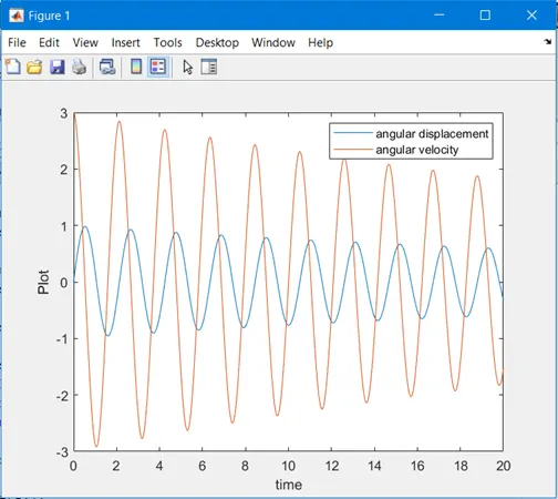
• We define the inputs for damping coefficient (b) , gravity (g), length (l), mass (m).Then we provide the initial condition for theta0 =[0;3]; where 0 is initial displacement and 3m/s is initial velocity .
• We next integrate the ode system to obtain a solution for which we need to assign the value for time which is tspan (it is a time array which goes from 0 – 20 seconds) with 500 values between them.
• Ode45 function is an inbuilt matlab solver, the variables being t and theta. Ode func is a separate matlab function which is t,theta,b,g,l and m are input parameters,

The first ode is given by

dθ/dt =dθ₁ /dt = θ₂

An the second ode is defined by

dθ₂/dt = -b/m θ₂ - g/l sinθ₁

• The odefunc code gives the integration of time and results.
• The result is a column vector which gives us displacement and velocity.
• By using the plot command graph was plotted between angular velocity and angular displacement with respect to time.

Program to create an animation of a simple pendulum

clear all

close all

clc

b=0.05;

g=9.81;

l=1;

m=1;

%initial condition

theta0 =[0;3];

%time points

tspan=linspace(0,20,500);

%solve ode

[t,results]=ode45(@(t,theta) odefunc(t, theta, b,g,l,m),tspan, theta0);

plot(t,results(:,1))

hold on

plot(t,results(:,2))

hold off

ylabel('Plot')

xlabel('time')

legend('angular displacement','angular velocity')

ct=1;

for i=1:length(results(:,1))

x0=0;

y0=0;

x1= 1*sin(results(i,1));

y1= -1*cos(results(i,1));

%simulation of simple pendulum

plot([x0 x1],[y0 y1],[-1 1],[0 0],'linewidth',3)

hold on

plot(x1,y1,'marker','o','markersize',25,'markerfacecolor','r')

axis([-1.5 1.5 -1.5 1])

grid on

title('motion of simple pendulum with damping')

pause(0.01)

M(ct)= getframe(gcf);

hold off

ct=ct+1;

end

%animation of motion of simple pendulum

movie(M)

videofile=VideoWriter('simplependulum.avi','uncompressed AVI');

open(videofile)

writeVideo(videofile,M)

close(videofile)

function code :

function[dthetadt]=odefunc(t,theta,b,g,l,m)

theta1=theta(1)

theta2=theta(2)

dtheta1dt=theta2

dtheta2dt=-(b/m)*theta2-(g/l)*sin(theta1);

dthetadt=[dtheta1dt;dtheta2dt];

end

EXPLANATION OF CODE:

• In order to run this program a counter is initiated. .
• For loop is creates a repetitive results displayed 500 times and hence an animation is generated
• To determine the co-ordinates we assume x0,y0 as (0,0) and using the geometric relations we consider x1 as 1*sin(results(i,1)) and y1 as -1*cos(results(i,1))
• Using the array brackets the string of the bob and the wall is plotted.
• Using the marker ‘0’ command the bob of the pendulum is created.
• It is slowed down to (0.01)
• A current frame command and movie command is written to create and animation in an uncompressed format

ERRORS:

1. In line 35 the error was y1= 1*cos(results(i,1)) when I did not put the minus sign it was found that the oscillation of the pendulum was inverted .

To rectify the mistake minus sign should be inserted y1= -1*cos(results(i,1)) for proper oscillation of the pendulum .

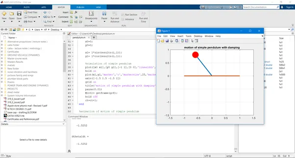
1. In the line 40 by mistake I put zero instead of ‘o’ .this created an error in creating bob for the pendulum

To rectify this mistake I replaced zero with ‘o’.

RESULTS:

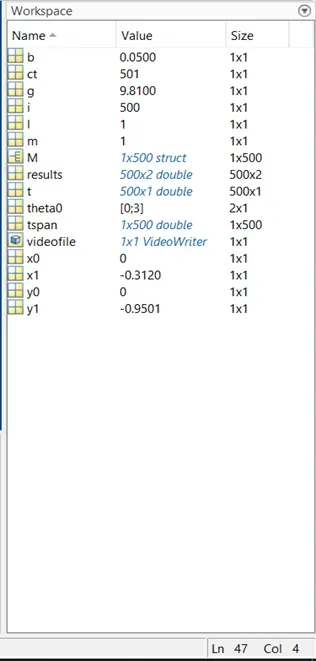
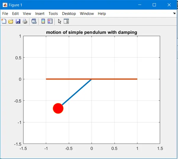
CONCLUSION:

Using the function ode 45, we can convert second order ode into first order ode to run the results.

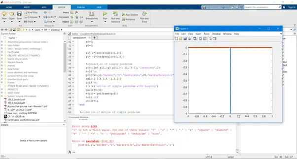
Thus, the simulation of transient behaviour of simple pendulum was successfully created using matlab.

Please note this is the video link (for the motion of the pendulum):

https://youtu.be/gFdIvPKgpK4

Program to solve second order differential equation.

clear all
close all
clc
 
b=0.05;
g=9.81;
l=1;
m=1;
 
%initial condition
 
theta0 =[0;3];
 
%time points 
tspan=linspace(0,20,500);
 
%solve ode
[t,results]=ode45(@(t,theta) odefunc(t, theta, b,g,l,m),tspan, theta0);
 
plot(t,results(:,1))
hold on
plot(t,results(:,2))
ylabel('Plot')
xlabel('time')
legend('angular displacement','angular velocity')

 
function[dthetadt]=odefunc(t,theta,b,g,l,m)
 
theta1=theta(1)
theta2=theta(2)
dtheta1dt=theta2
dtheta2dt=-(b/m)*theta2-(g/l)*sin(theta1);
dthetadt=[dtheta1dt;dtheta2dt];
end



 
Program to create an animation of a simple pendulum


clear all
close all
clc
 
b=0.05;
g=9.81;
l=1;
m=1;
 
%initial condition
 
theta0 =[0;3];
 
%time points 
tspan=linspace(0,20,500);
 
%solve ode
[t,results]=ode45(@(t,theta) odefunc(t, theta, b,g,l,m),tspan, theta0);
 
plot(t,results(:,1))
hold on
plot(t,results(:,2))
hold off
ylabel('Plot')
xlabel('time')
legend('angular displacement','angular velocity')


ct=1;
for i=1:length(results(:,1))
x0=0;
y0=0;

x1= 1*sin(results(i,1));
y1= -1*cos(results(i,1));

%simulation of simple pendulum
plot([x0 x1],[y0 y1],[-1 1],[0 0],'linewidth',3)
hold on
plot(x1,y1,'marker','o','markersize',25,'markerfacecolor','r')
axis([-1.5 1.5 -1.5 1])
grid on
title('motion of simple pendulum with damping')
pause(0.01)
M(ct)= getframe(gcf);
hold off
ct=ct+1;
end

%animation of motion of simple pendulum
movie(M)
videofile=VideoWriter('simplependulum.avi','uncompressed AVI');
open(videofile)
writeVideo(videofile,M)
close(videofile)


function code :

function[dthetadt]=odefunc(t,theta,b,g,l,m)
 
theta1=theta(1)
theta2=theta(2)
dtheta1dt=theta2
dtheta2dt=-(b/m)*theta2-(g/l)*sin(theta1);
dthetadt=[dtheta1dt;dtheta2dt];
end



Please note this is the video link (for the motion of the pendulum):
https://youtu.be/gFdIvPKgpK4