Week 4.1 - Genetic Algorithm

Aim :

• To write a code in MATLAB to optimize Stalagmite Function using Genetic Algorithm (GA) and find its global maxima.
• To explain the concept of Genetic Algorithm and also the syntax used for GA in MATLAB.
• To sure make that the code gives the same output, even if it is made to run several times.
• Plot graphs for all the 3 studies and for Fmaximum v/s No. of iterations.

Governing Equations :

The below relations were used while coding the Stalagmite Function :

`f (x,y )= -(f1,x*f2,x*f1,y*f2,y)

f1,x= [sin(5.1πx+0.5) ]^6

f1,y=[sin(5.1πy+0.5 ) ]^6

f2,x= exp[-4ln2* (x-0.0667 )^2 /0.64]

f2,y=exp[-4ln2*(y-0.0667 )^2 /0.64]`

Since the ga always minimizes a function, but, our objective is to find the maxima,so by inverting the Stalagmite Function by adding a minus sign will give the minimum values.And at last,taking the magnitude of the peak negative value will give us the maxima.

Genetic Algorithm :-

Genetic Algorithm is an optimization technique used to find optimal or near optimal solutions.It is based on Evolution Theory proposed by Charles Darwin.

Working of Genetic Algorithm (GA) :-

• Population Initialization :- In the 1^st step,algorithm begins by creating random initial population and if you know approximately where the minimum point for the function lies,you can set the initial population range such that the point lies in the middle of that range
• Population is the no. of sample data points chosen to perform GA.
• At each step the GA uses the current population to create children that make up the next generation.
• Selection :-In this,parents are selected from the random sample points and the main objective of this step is to select the fittest individuals by assigning the fitness value in accordance to fitness functions.
• We can specify the fitness function that the algorithm uses to select the parents in the Selection Fcn
• The fittest value will have the higher probability in the Roulette Wheel and from this step parents are selected for the Cross-over process.
• Crossover :- It is the process of choosing 2 parents and the producing the children from them by interchanging their genes i.e., entries of their vector.
• Mutation :- Mutation is carried out in order to maintain the genetic diversity from one generation of population to the next.In this process,the genes will be replaced by some random integer.
• If mutation is not done ,the genes will become similar to each other,converging to a local minima.
• Mutation and Cross-over explains how to specify the no. of children of each type that the algorithm generates and the function it uses to perform cross-over and mutation.
• The above process of Selection-Crossover-Mutation is repeated for the new child until an optimised result is found out.
• Termination Condition of Algorithm :- The ga uses the options to determine when to stop.See the default values for each option by running options = optimoptions(‘ga’).
• The algorithm stops as soon as any one of the conditions is met.

Syntax for Genetic Algorithm in MATLAB :-

• x = ga(fun,nvars) : finds a local unconstrained minimum x,to the objective function x.where fun is the objective function and nvars is the no.of variables.
• x = ga(fun,nvars,A,b) : finds a local minima x to function(fun) subject to linear inequalities A*x ≤ b.Evaluating the matrix product A*x,as if x is transposed (x’).
• x = ga(fun,nvars,A,b,Aeq,beq) : finds local minima to the function subject to linear equalities Aeq*x=beq and A*x ≤ b.(Set A,b = [],if no linear inequalities exist). Evaluating the matrix product Aeq*x,as if x is transposed (x’).
• x = ga(fun,nvars,A,b,Aeq,beq,lb,ub) : bounding the range of x, between upper and lower bounds.(Set Aeq,beq = [],if no linear equalities exist).
• x = ga(fun,nvars,A,b,Aeq,beq,lb,ub,nonlcon) : minimizes x wrt the options in nlcon (non-linear constraints).(Set lb,ub = [] if no bounds exists).
• x = ga(fun,nvars,A,b,Aeq,beq,lb,ub,nonlcon,options) : minimizes x with the default optimization parameters replaced by values in options.(Set nonlcon =[] if no nonlinear constraints.Create options using
• x = ga(fun,nvars,A,b,Aeq,beq,lb,ub,nonlcon,intcon) : here the variables in intcon (integer constrain) takes integer values.
• x = ga(fun,nvars,A,b,Aeq,beq,lb,ub,nonlcon,intcon,options)
• x = ga(problem) : finds the minimum for problem.The problem is described containing the below fields :

fitnessfcn-Fitness functions

nvars-Number of design variables

Aineq-A matrix for linear inequality constraints

Bineq-b vector for linear inequality constraints

Aeq-Aeq matrix for linear equality constraints

Beq-beq vector for linear equality constraints

lb-Lower bound on x

ub-Upper bound on x

nonlcon-Nonlinear constraint functions

intcon -Indices of integer variables

rngstate-Field to reset the state of the random number generator

solver -'ga’

option-Options created using optimoptions or an options structure

We must specify the fields fitnessfcn, nvars, and options. The remainder are optional for ga.

• [x,fval] = ga(___) :for any previous input arguments,also returns fval(fitness function value at x.
• [x,fval,exitflag,output] = ga(___) : also returns exitflag, an integer identifying the reason the algorithm terminated, and output, a structure that contains output from each generation and other information about the performance of the algorithm.
• [x,fval,exitflag,output,population,scores] = ga(___) : also returns a matrix population, whose rows are the final population, and a vector scores, the scores of the final population.

MATLAB Code :-

clear all
close all
clc

x = linspace(0,0.6,150);
y = linspace(0,0.6,150);

% Running 50 iterations (ie.,Initial Population Size is set to 50 by default)
num_cases = 50 ;

% Creating a 2D array/mesh with 1-D array (i.e., Generating 2-D domain for
% the Stalagmite Function
[xx,yy] = meshgrid(x,y);

% Creating the Stalagmite Function using xx & yy values
f = get_stalagmite(xx,yy);

% Evaluating the stalagmite function
% for loops is generating the data for stalagmite function
tic
% Study1 - Statistical Behaviour
for i = 1:num_cases  
    [inputs,fopt(i)] = ga(@stalagmite,2);
    xopt(i) = inputs(1);
    yopt(i) = inputs(2);
end
study1_time = toc

figure(1)
subplot(2,1,1)
hold on 
surfc(xx,yy,f)
shading interp
plot3(xopt,yopt,fopt,'marker','o','markersize',5,'markerfacecolor','r')
title('Unbounded Inputs')
subplot(2,1,2)
plot(fopt)
xlabel('No. of Iterations')
ylabel('Function Minimum')

tic
% Study2 - Statistical behaviour with lower & upper bounds
for i = 1:num_cases
    [inputs,fopt(i)] = ga(@stalagmite,2,[],[],[],[],[0;0],[1;1]);
    xopt(i) = inputs(1);
    yopt(i) = inputs(2);
end
study2_time = toc

figure(2)
subplot(2,1,1)
hold on 
surfc(xx,yy,f)
shading interp
plot3(xopt,yopt,fopt,'marker','o','MarkerSize',5,'MarkerFaceColor','r')
title('Bounded Inputs')
subplot(2,1,2)
plot(fopt)
xlabel('No. of Iterations')
ylabel('Function Minimum')


%Study3- Increasing GA iterations(Increases the simulations time due to increased population size) 
% Lesser population size results in local minimas rather than a global
% minima
options = optimoptions('ga');
options = optimoptions(options,'PopulationSize',300);

tic
for i = 1:num_cases
[inputs,fopt(i)] = ga(@stalagmite,2,[],[],[],[],[0;0],[1;1],[],[],options);
xopt(i) = inputs(1);
yopt(i) = inputs(2);
end
study3_time = toc
figure(3)
subplot(2,1,1)
hold on 
surfc(xx,yy,f)
shading interp
plot3(xopt,yopt,fopt,'marker','o','MarkerSize',5,'MarkerFaceColor','r')
title('Bounded Inputs with Increased Population Size')
subplot(2,1,2)
plot(fopt)
xlabel('Iterations')
ylabel('Function Maximum')

z = abs(fopt);



% Due to more population size the simulation time increases bcoz the GA processes 
% more no. of individuals,you need to process them & also evaluate the function    

Workflow of the code :

• Firstly,we define 2 input arrays/vectors named as x & y and in that we’d put 150 numbers between 0 & 0.6 using linspace command.
• Then,we defined the initial population size to 50,which is also the no. of times the iterations is going to run.
• Creating 2-D domain or array/mesh for the function from 1-D x & y input vectors using meshgrid command.
• Creating the Stalagmite Function.
• Now,the optimization of Stalagmite Function using GA is evaluated here based on 3 studies.
• In 1^st Case Statistical Behaviour of GA is studied in which our Optimization Algorithm i.e., Genetic Algorithm uses initial population as 50.
• for loop is used to check all 50 population samples.
• Now,the ga (Genetic Algorithm) is employed using the appropriate syntax and passing in 2 inputs i.e.,the stalagmite function by usage of function handle and the 2 inputs to the stalagmite function i.e., x & y.
• Storing these 2 inputs x & y to two variables i.e., xopt(i) and yopt(i) and closing the loop and lastly adding tic and toc commands for calculating the study time taken by the algorithm.
• figure command is used to open figure window.
• Subplot command is used to generate multiple plots inside the same figure window and here it is divided into 2 subplots.
• surfc command generates the 3D stalagmite function model in the 1^st
• shading interp command removes the grid lines generated on the plot,making it smooth.
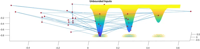
• plot3 command is used to plot the xopt,yopt & optimum function (fopt) values that GA predicts over 50 studies in subplot 1 which will help us visualize how the algorithm is performing .
• title is to the figure 1 is given as ‘Unbounded Inputs’.
• 2^nd subplot is accessed & inside the 2^nd subplot,optimum function value (fopt) is directly generated over 50 studies using plot command.
• Now,as Genetic Algorithm works on Random Sampling,so we get different outputs from the code everytime it’s executed.So,1^st study can’t be used for optimization for getting the maxima of the function and it shows the function value (fopt) in the range of [-1,0].
• In 2^nd Study, we set the bounds of input variables by changing the syntax and containing the values between 0 & 1 i.e., in a square of unit length.
• So,in this case the minimum values lies between 4 peaks and the functional values obtained in this case is between [-1,-0.7),which is a more narrow range.
• In 3^rd study,in addition to setting the bounds we’re also increasing the Population size i.e., increasing GA iterations using optimoptions command.
• Optimoption command is used to create optimization options.
• [Syntax used :- options = optimoptions(Solvername) returns a set of default options for the Solvername solver.
• Syntax used for setting population size :- options = optimoptions(options,’PopulationSize’,300).
• On increasing the population size to 300,the algorithm converges the optimum function value (fopt) to -1 which is the global minima of the Stalagmite Function as evident from the figure.
• But,here in this problem we want the global maxima,so using ‘abs’ function to get the magnitude of absolute/peak value.

Function Code 1 :

% get_stalagmite function is generating the stalagmite function by sending
% each data to input variable 
function f = get_stalagmite(xx,yy)
for i = 1:length(xx)
    for j = 1 :length(yy)
    input(1) = xx(i,j);
    input(2) = yy(i,j);
    f(i,j) = stalagmite(input);

    end
end

Function Code 2 :

function [f] = stalagmite(input)

x = input(1);
y = input(2);
term1 = (sin(5.1*pi* x + 0.5)).^6 ;
term2 = (sin(5.1*pi* y + 0.5)).^6 ;
term3 = exp (-4*log(2) * (( x - 0.0667).^2) / 0.64 ) ;
term4 = exp (-4*log(2) * (( y - 0.0667).^2) / 0.64 ) ;

f = - (term1 * term2 * term3 * term4) ;

end

Output Plots :

Study 1:

-

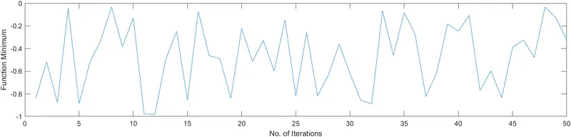
Study1_time = 4.7976 s

Study 2 :-

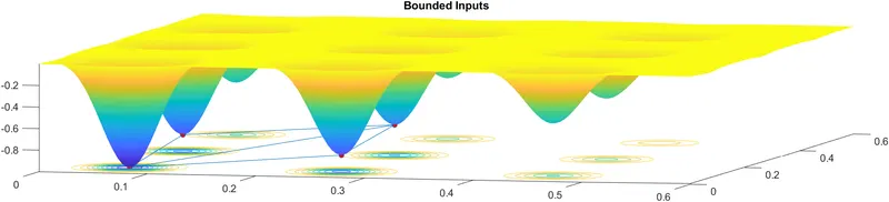
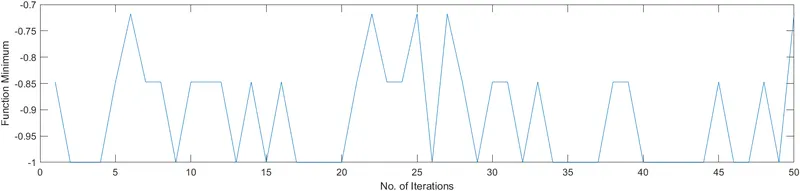
Study2_time = 5.9666 s

Study 3 :-

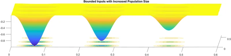
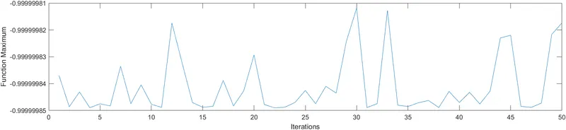
Study3_time = 19.3390 sec

Errors :

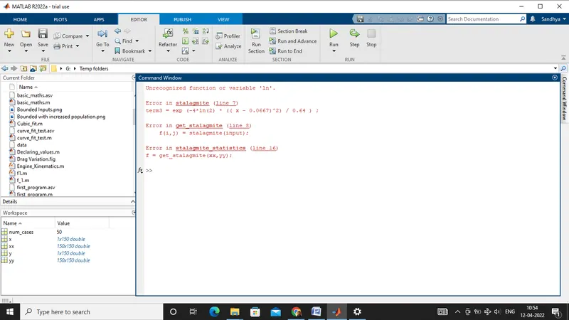
Steps taken to overcome the errors :

• Usage of log() function for returning the natural logarithm value.As in MATLAB it is defined in this manner which is like the conventional way of defining the log function with 10 base.

Conclusion :

• The above studies shows that the Optimization using Genetic Algorithm is a rigorous iterative process for getting the optimal solutions.
• The last study took almost 4 times than the 1^st study i.e.,5 sec and tells us that the genetic algorithm slows down when the initial population is increased and takes times for the convergence.
• Global Maxima (fopt) = 1.