Week 3 - Solving second order ODEs

objective:

To write a program that solves the following ODE and to create the animation of a simple pendulum.

• This ODE represents the equation of motion of a simple pendulum with damping

explanation:

1. ODEs (ordinary differential equations)are used to define the behavior of the systems by using dependent and independent variables. the above equation represents the behavior of a simple pendulum with time as an independent variable and theta as the dependent variable
2. generally while solving ODE equations computationally by using Matlab there are some rules
3. only first-order ODE can be solved
4. In the case of higher-order ODEs, we should convert them into first-order odes.
5. these converted higher-order ODEs should be represented in array form in Matlab.

• solving ode in Matlab

the second-order differential equation we are supposed to solve is derived for a simple pendulum on the application of Newton's second law.

before writing a program we should convert higher order ode into first-order ode as follows

`(d^2theta)/dt^2+b/m*(d theta)/dt+(g/l)sin(theta)`=0`

`theta=theta1`

`(d theta)/dt=(d theta1)/dt=theta2` equation 1

`(d^2theta)/dt=(d^2theta1)/dt^2=d/dt((d theta1)/dt)=(d theta2)/dt`

`(d^2theta)/dt^2+b/m*(d theta)/dt+(g/l)sin(theta)`=0`

`(d^2theta)/dt^2+b/m*(d theta1)/dt+(g/l)sin(theta)`=0`

`(d theta2)/dt+b/m*theta2+g/l*sin(theta1)=0`

`(d theta2)/dt=b/m*theta2+g/l*sin(theta1)` equation 2

we represent these two equations in matrix form

`d/dt((theta1 ),(theta2))=((theta2),(-b/m*theta2-g/l*sin(theta1)))`

• while writing program we represent left hand side of equation with 'theta'

step vise explanation of program

step1:

first create function definition in matlab by using above equations.as shown bellow

% function for solvation of ode for time and  mass system in simple pendulum
function [dtheta]=doc_fuc(t,theta,b,g,m,l)
 theta1=theta(1);  %angular displacement in solution set
 theta2=theta(2);    %angular velocity
 dtheta1_dt=theta2;  %1st equation
 dtheta2_dt=(-b/m)*theta2-(g/l)*sin(theta1);   %second equation
 dtheta=[dtheta1_dt;dtheta2_dt]     %solution set
end

step2:

open the new script, enter initial values where theta as a variable which includes angular displace meant and angular velocity and

time interval

step3:

Use the ode45 command to solve the first-order differential equations

Syntax:ode45(@(independent variable, dependent variable) function definition, time, initial conditions)

In this syntax first, we define variables, and functions then provide inputs.

As we have two equations we get two outputs i. e., time and results which include angular displacement and angular velocity with respect to time values. In the form of an array with size mx2.

step4:

we use the following information to plot graphs between time, angular displacement, and angular velocity.

to visualize how data is changing with respect to one other.

% solving ode representing simple pendulum for graphical representation of time, angular displacement, and angular velocity. 

close all    %closes all graphical windows open
clear all    %clears workspace
clc           %clears command window

% inputs
g=9.81  %gravitational accelaration (m/sec^2)
b=0.05    %damping co-efficient
l=1       %string length(m)
m=1        %mass of bob(kg)

%initial 
theta=[0;3];   %values of angular displacement and velocity at t=0

%time span
t_span=linspace(0,20,150);

%ode solvation

[t,results]=ode45(@(t,theta) doc_fuc(t,theta,b,g,m,l),t_span,theta);%ode45 is an inbuilt function used to solve first order differential euations
   %as we have two 1st order ode equations we get two solutions
   
   
%plots
figure(1)
hold on    %this command to avoid over writting of plots
axis([0 25 -4 4])   %defining x and y axis limits
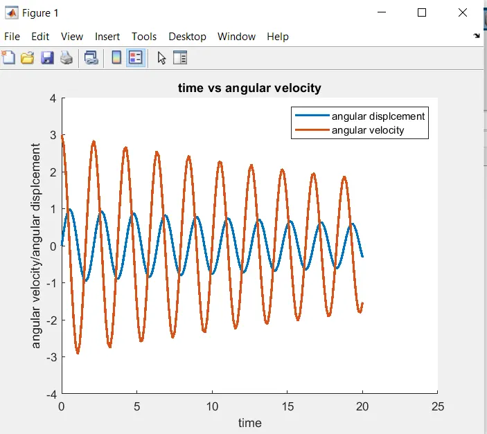
plot(t,results(:,1),'linewidth',2)  %plot between time anfd angular displacement
plot(t,results(:,2),'linewidth',2)  %plot between time and angular velocity
title('time vs angular velocity')  
legend('angular displcement','angular velocity')  % through this we can name the line ploted on graph

%reprasentation of AXIS
xlabel('time') 
ylabel('angular velocity/angular displcement')

results1: motion of simple pendulum having damping coefficient 0.05 with respect to time.

2.

• program for animation of pendulum

step1:

first, solve the ode equation given as mentioned above

step2:

output after solving the ode is used for animation. so that consider a variable let as 'i', with the condition of 'i=0:length(t_span)'by using this condition under for loop so that I can iterate the commands under loop up to the required number.

step 3:

• considered (x0,y0) as the hinge point,from geometrical calculation obtainedx1=`l*sin(theta)`

`y1=-l*cos(theta)`

• here for simplification consider 'theta=results(i,1)', it represents that for every iteration of 'i' value theta will be overwritten with value of angular displace meant which is stored under variable called results after solving ode equation.
• by using x1 and y1 values we can locate the bob position.

step4:

• represent the dataset on the graph by using the plot command. it must use the hold-on command to avoid overwriting graphs at every iteration.

step5:

after all, it's time to create an animation using all the graphs.

• consider a variable to store all graphs together
• using the 'movie(variable)' command preview of animation is created.
• to save this animation use 'videowrite('file name.avi','type of file')'.
• open the file created with the help of open(filename), then store the information into it by 'writevideo(filename, variable)'.after all is done close the file.

link:

YouTube link for simple pendulum animation

program:

%creation of simple pendulum animation by solving second order ode equation
%which represents the motion of the simple pendulum

close all         %closes all graphical windows open
clear all          %clears workspace
clc                %clears command window

% inputs
g=9.81  %gravitational accelaration (m/sec^2)
b=0.05    %damping co-efficient
l=1       %string length(m)
m=1        %mass of bob(kg)


%initial conditions at meeen position t=0
theta=[0;3];

%time span
t_span=linspace(0,20,150);
%hing position of pendulam
x1=0;
y1=0;

ct=1;

%ODE solvation for representing the motion of the pendulum.

 [t,results]=ode45(@(t,theta) doc_fuc(t,theta,b,g,m,l),t_span,theta); %ode45 is an in built function in matlab used to solve 1st order differencial equations
 %logic for animation creation
 
for i=1:length(t_span) %i value is onsidered untill the llenght of t_span
    THETA=results(i,1); % at perticulsr value of i  results(i,1) reprasents angula displacement
    
    %co-ordinates for second end of string
    x2=l*sin(THETA);
    y2=-l*cos(THETA);
    
    %plot
    figure(ct)     
    hold on
    grid on
    
    plot(x1,y1,'marker','+')  %hinge position
    line([x1,x2],[y1,y2],'linewidth',2,'color','r')  %string
    plot(x2,y2,'marker','o','markerfacecolor','k','markersize',10)  %positioning of bob
    line([0 0],[0 -1.1],'linewidth',2,'linestyle','--','color','k')  %meen position line reprasentation for refference
    line([-0.8 0.8],[0 0],'linewidth',4)  % support to hing the pendulam
    axis([-2 2 -1.5 1.5]);   %defining axis limits
    title('simple pendulam animation') % to display title on the graphical window
    
    % representation x and y axis
    xlabel('x-axis')
    ylabel('y-axis')
    
    s(ct)=getframe(gcf);   %all frames are stored in s by forming 's' as a stuct
    ct=ct+1;
end

%movie creation
  movie(s)      %crestes the animation  with the frames collected
  videofile=VideoWriter('simple_pendulam.avi','uncompressed AVI');  %vedio is created with the name of simple_pendulam
  videofile.FrameRate=5  %no of frames to be displayed per second while creating a video through this duration of video created is calculated
  open(videofile)       %open video file to edit
  writeVideo(videofile,s)  % information is loaded in to the file created through the write video command 
  close(videofile)  %after editing close the file

errors

1. hear ode is solved under for loop

therefore doe is solved before for loop by using ode45.

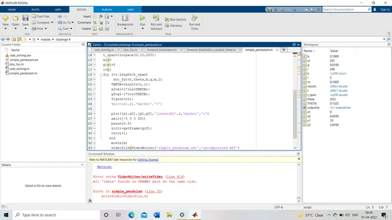
2. 'figure(ct)' command is used after plot commands, as I replace it to before plot commands,I was able to create the animation.