Week 4.1 - Genetic Algorithm
Aim:-optimization of stalagmite function using genetic algorithm in Matlab.
stalagmite:-
- the physical appearance of stalagmite is a type of rock formation that rises from the floor of a cave due to the accumulation of material deposited on the floor from ceiling drippings.
- function representing the shape of the stalagmite called as stalagmite function.
- A stalagmite function generally refers to the function with which we are generating values over a stalagmite kind of surface for finding out the local and global maxima and minima of that particularly given function. For this, we are using a method called 'Optimization'.
`f(x,y)=f_1*_xf_2*_xf_1*_yf_2*_y`
`f_1*_x=[sin(5.1*pi*x+0.5)]^6`
`f_1*_y=[sin(5.1*pi*y+0.5)]^6`
`f_2*_x=exp[-4*ln(2)*(((x-0.0667)^2)/0.64)]`
`f_2*_y=exp[-4*ln(2)*(((y-0.0667)^2)/0.64)]`
optimization:-
- it can be defined as the best outcome from the set of different combinations of input values.
- some times best outcome in the sense of optimization is maximizing or minimizing one or more objective functions, by varying the input parameters.
- optimization can be done in different ways through computation one of them is the genetic algorithm.
genetic algorithm
- genetic algorithm was introduced by john holland in early 1970
- it is the search-based algorithm used for solving optimization problems.
- this technique is inspired by Charles darwin's theory of evolution. according to him
''it is not the strongest of the species that survive,
nor the most intelligent, but the one most responsive to change.''
consider the following example to understand how the above quote gives birth to the genetic algorithm concept
ex:-
suppose, we have 100 people consisting of 50 men and 50 women now, suppose all the 100 people get married and give birth to other 50 children. these 50 children will have the best qualities of their parents. now suppose out of these 50, again there are 25 boys and 25 girls. now, these 25 boys and 25 girls are selected for the next process to find the healthiest and most intelligent child. for these purposes, these are married again and give birth to 25 other children. now, these 25 children will have the again the best genetically surviving qualities of their parents as well as some other good qualities. this process is continued till we get a single child. which is the best healthiest and most intelligent among all this whole process is called the natural evolution of humans.
- the genetic algorithm basically follows this idea.
- this algorithm reflects the process of natural selection where the fittest individuals are selected for reproduction in order to produce offspring(children) of children of the next generation. therefore the process of natural selection starts with the selection of the fittest individuals from the population. they produce offsprings that inherit the characteristics of the parents and will be added to the next generation. if parents have better fitness, their offspring will be better than their parents and have a better chance of surviving. this process keeps on iterating and in the end, generation with the fittest individual will be found.
- this idea can be applied for a search problem related to any engineering field or optimization filled
- we consider a set of solutions for a problem and select the set of best out of them.
step by step process how genetic algorithm transforms biological process to mathematical and optimizations process.
- initialization or initial population
- fitness function
- selection
- crossover(recombination)
- mutation
- Initialization or initial population
the genetic algorithm starts with generating an initial population. the initial population consists of a set of individuals in which each individual is a solution to the problem that needs to be solved.
the individual is characterized by a set of parameters(variables) known as genes and the genes are joined into a string to form a chromosome(solution). the chromosome is basically one of the possible solutions.
chromosome=possible solutions, results, answer
quality, or characteristics of the chromosome (solution)depend upon the quality(fitness) of the genes(variables or parameters).
- Fitness function:-
after the initialization of the population, we determine the ability of the individual to compete with other individuals by using the fitness function. the fitness function determines how to fit an individual or in other words how close it is to the best solution. let's suppose if we are minimizing the error, the best fittest individual will be that which has. the lowest error among all. this is obtained by assigning the fitness score to each individual. this is a necessary process because the probability of an individual will be selected for reproduction or shifted to the next step depends upon the fitness score. higher the fitness score, the higher the chances of being chosen for reproduction and vice versa.
- selection:-
in this phase, individuals are selected again for the reproduction of offspring. the selected individuals are arranged in pairs of two to enhance reproduction. these individuals pass on their genes to the next generation.
the main aim of this phase is to establish the region with a high chance of generating the best solution to the problem better than the previous generation.
- crossover
crossover is the most significant phase in a genetic algorithm. for each pair of parents to be mated, a crossover point is chosen at random from within the genes
or
- The algorithm creates crossover children by combining pairs of parents in the current population. At each coordinate of the child vector, the default crossover function randomly selects an entry, or gene, at the same coordinate from one of the two parents and assigns it to the child. For problems with linear constraints, the default crossover function creates the child as a random weighted average of the parents.
- Mutation
are the children produced have the exact same qualities as their parents? no., there must be some changes in the genes of children during their growth which makes them different from their parents. this process is known as mutation.
then it is said that the genetic algorithm has provided a set of solutions to our problem. the population has a fixed size. as the new generations are formed, individuals with the least fitness die, providing space for new offspring. the sequence of phases is repeated to produce individuals in each generation who are better than the previous generation. ga as a function of Matlab
sintax of ga:-
x = ga(fun,nvars)x, to the objective function, fun. nvars is the dimension (number of design variables) of fun.
Note
Passing Extra Parameters (Optimization Toolbox) explains how to pass extra parameters to the objective function and nonlinear constraint functions, if necessary.
x = ga(fun,nvars,A,b,Aeq,beq,lb,ub,nonlcon)nonlcon. The function nonlcon accepts x and returns vectors C and Ceq, representing the nonlinear inequalities and equalities respectively. ga minimizes the fun such that C(x) ≤ 0 and Ceq(x) = 0. (Set lb=[] and ub=[] if no bounds exist.)
x = ga(fun,nvars,A,b,[],[],lb,ub,nonlcon,IntCon)x = ga(fun,nvars,A,b,[],[],lb,ub,nonlcon,IntCon,options)IntCon take integer values.
Note
When there are integer constraints, ga does not accept linear or nonlinear equality constraints, only inequality constraints.
fval, the value of the fitness function at x.to the objective function, fun. nvars is the dimension (number of design variables) of fun.- considered variables of x and y assigning with input parameters
- create 2d arrays by using mesh grid to represent a function in 3d
- then create a loop for solving function with given inputs. these solutions that we are getting are stored in a variable called 'f'.this is called initialization of population.
- code for a function to be optimized
-
% stalagmite function function [f1]=func(interval) x=interval(1); y=interval(2); f_1= (sin((5.1*pi*x)+0.5)).^6; f_2= (sin((5.1*pi*y)+0.5)).^6; f_3= exp(-4*log(2)*(((x-0.0667).^2)/0.64)); f_4= exp(-4*log(2)*(((y-0.0667).^2)/0.64)); f1= -((f_1).*(f_2).*(f_3).*(f_4)); end - then by using the 'ga' function which is inbuilt in Matlab for solving search based optimization problems to get the optimum value of the function
- in stalagmite function we multiply with the negative sign because using 'ga' will return minimum value of the function. so that we can manage to calculate the maximum value in return.
- actually in below code include the representation stalagmite function and 3 studies with different inputs to 'ga' and plots between function maximum vs iterations to represent how the ga is performing.
- in 3 study we are using 'optimization('solver name')' to get default options i.e,size of population.
- 'options=optimoptions(old options,name,value)'returns a copy of
oldoptionswith the named parameters altered with the specified values. - By increasing the population we are increasing the no of solutions so that scope of finding optimal value increases.
- every time I increase the inputs to 'ga' it will increase my study time.
Stopping Conditions for the Algorithm
The genetic algorithm uses the following options to determine when to stop. See the default values for each option by running opts = optimoptions('ga').
-
MaxGenerations— The algorithm stops when the number of generations reachesMaxGenerations. -
MaxTime— The algorithm stops after running for an amount of time in seconds equal toMaxTime. -
FitnessLimit— The algorithm stops when the value of the fitness function for the best point in the current population is less than or equal toFitnessLimit. -
MaxStallGenerations— The algorithm stops when the average relative change in the fitness function value overMaxStallGenerationsis less thanFunction tolerance. -
MaxStallTime— The algorithm stops if there is no improvement in the objective function during an interval of time in seconds equal toMaxStallTime. -
FunctionTolerance— The algorithm runs until the average relative change in the fitness function value overMaxStallGenerationsis less thanFunction tolerance. -
ConstraintTolerance— TheConstraintToleranceis not used as a stopping criterion. It is used to determine the feasibility with respect to nonlinear constraints. Also,max(sqrt(eps),ConstraintTolerance)determines feasibility with respect to linear constraints.
The algorithm stops as soon as any one of these conditions is met
program
close all     %closes all the graphical windows
clear all      %clear the workspace
clc            %clears the command window


%input variables
x=linspace(0,0.6,150);
y=linspace(0,0.6,150);
%creating meshgrid for 3d plot
[xx yy]=meshgrid(x,y);

%loop for solving function each variable
for i=1:length(xx)
    for j=1:length(yy)
        interval(1)=xx(i,j);
        interval(2)=yy(i,j);
        f(i,j)=func(interval);
    end
end
hold on
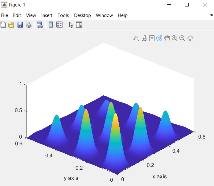
%reprasentation of stalagmite function by using surf command
figure(1)
surf(xx,yy,-f);
xlabel('x axis');
ylabel('y axis')

shading interp  % this command will make the plot smooth


%% study 1 statistical behavior of ga function
%use x and y values as mentioned above
num_case=200;   %by providing num_case we actually running the ga function 200 times

tic           %tic command starts the timer
for i=1:num_case
    %in this study we first we define the function and give no of individual variables
    [inputs,fopt(i)]=ga(@func,2);  %here 'inputs' include the x and y co ordinates of that 'fopt'(optimum values) obtained.
    xopt(i)=inputs(1);
    yopt(i)=inputs(2);
end
study1_time=toc     %toc command stops the timer
%poltting
figure(2)
subplot(2,1,1);   %subplot is used to reprasent two graphs in one figure
title('unbounded serch space')
hold on
surf(x,y,-f);
xlabel('x axis')
ylabel('y axis')
shading interp
plot3(xopt,yopt,-fopt,'marker','o','markersize',5,'markerfacecolor','r');  %plot3 command used to plot points in 3d plot
subplot(2,1,2);
plot(-fopt)  %negitive sighn before 'fopt' is used to reprasent grapht in positive value it will not effect the results.
xlabel('iterations')
ylabel('function maximum')
hold off

%% study 2 optimization by providing limits or bounds
% hear  we consider upper and lower bounds of x and y between 0 to 0.6
%0<=x>=0.6 and 0<=y>=0.6
%in the second study we are defining the search space for optimum value, so that
%ga will calculate for optimum values in that range only
tic
for i=1:num_case
    [inputs,fopt(i)]=ga(@func,2,[],[],[],[],[0;0],[0.6;0.6]);  %ga function having some '[]'  brakets it means empty inputs for that variables according to the syntax
    xopt(i)=inputs(1);
    yopt(i)=inputs(2);
end
study2_time=toc
%plotting
figure(3)
subplot(2,1,1);
hold on
title('bounded serch space')
surf(x,y,-f);
xlabel('x axis')
ylabel('y axis')
shading interp
plot3(xopt,yopt,-fopt,'marker','o','markersize',5,'markerfacecolor','r');
subplot(2,1,2);
plot(-fopt)
xlabel('iterations')
ylabel('function maximum')


%% study 3 incresing  polupation size
%by changing the polpulation size from default to 600 we can increase the
%scope to serch for optimum value
options=optimoptions('ga');   % function stores the default population size into a variable
options=optimoptions(options,'populationsize',600);  %replacing default polpulation size with user defined polpulation size
tic
for i=1:num_case
    [inputs,fopt(i)]=ga(@func,2,[],[],[],[],[0;0],[0.6;0.6],[],[],options);
    xopt(i)=inputs(1);
    yopt(i)=inputs(2);
end
study3_time=toc
figure(4)
subplot(2,1,1);
hold on
title('bounded serch space with increse in population size');
surf(x,y,-f);
xlabel('x axis')
ylabel('y axis')
shading interp
plot3(xopt,yopt,-fopt,'marker','o','markersize',5,'markerfacecolor','r');
subplot(2,1,2);
plot(-fopt)
xlabel('iterations')
ylabel('function maximum')- 1st plot representation of stalagmite function
- 2nd plot
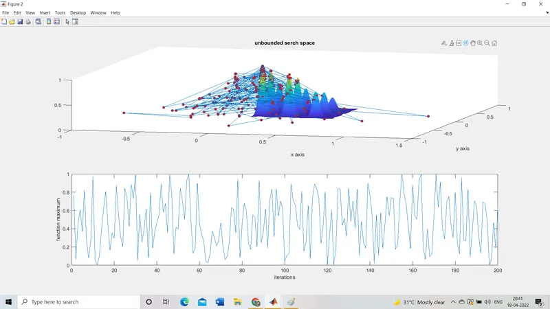
this plot represents different maximum values at every iteration it goes through with more differences in values and the values are plotted beyond the plot representing the stalagmite function. so that we go further by providing more no of inputs for accuracy
- 3rd plot
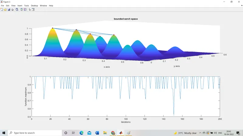
this plot gives results better than plot 2 i.e., the values are plotted in the function validation range. but in this also we are not getting accurate optimum values or the values we are getting are having more variability.
- 4th plot
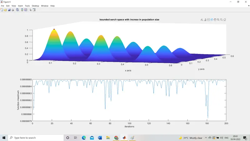
in this plot, we increased the population size for better results. but we are still not getting accurate optimum value but the range of variation between the values we get are negligible. so on average, we can consider 0.9999984 as the optimum value.
errors
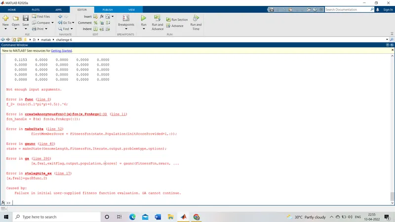
I got this error because while creating the function I created a function with 2 input variables while using this function in the main script I have given one input
I solve this by changing the no. of inputs in the function definition according to the main script.