Week 3: Flow over a backward facing step

SIMULATING FLOW OVER BACKWARD-FACING STEP

l. INTRODUCTION

The Backward-facing step is a standard geometry used for visualizing the recirculation flow and validating turbulence models. BFS flow is one representative model for separation flows, which is widely used in aerodynamic flows, condensers, vehicles, etc.

In this project, Converge studio was used to establish a working idea of airflow simulation through a backward-facing step under certain parameters, which will be established systematically in this project.

ll. OBJECTIVE

1. Setup backward-facing step flow simulation.
2. Run simulation for 3 different mesh sizes.
3. PLot Velocity and pressure contours for all 3 mesh sizes.
4. Show plots for velocity, pressure, mass flow rate, and total cell count for all 3 mesh sizes.

lll. PROCEDURE

GEOMETRY:

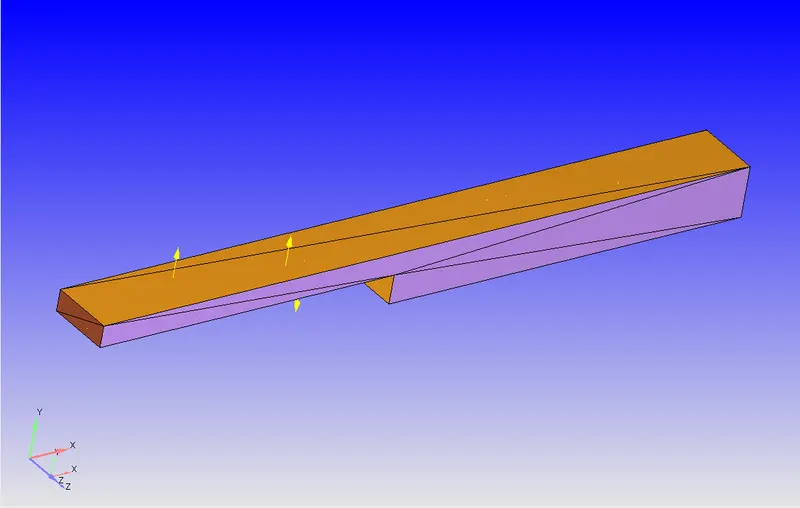
• Importing the downloaded geometry.
• Running diagnosis to check if there are any open edges or faces.
• Checking the orientation of Normals, the normals should be such that their orientation is pointing towards the fluid flow.

BOUNDARY FLAGGING:

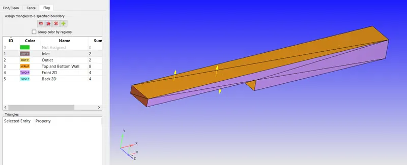
The boundaries are flagged. The converge studio basically uses triangular blocks to create geometry. So by selecting the triangles boundaries are Flagged.

• Inlet
• Outlet
• Top and Bottom Wall
• Front 2D
• Back 2D

CASE SETUP:

• Application Type = Time-based
• Material = Air
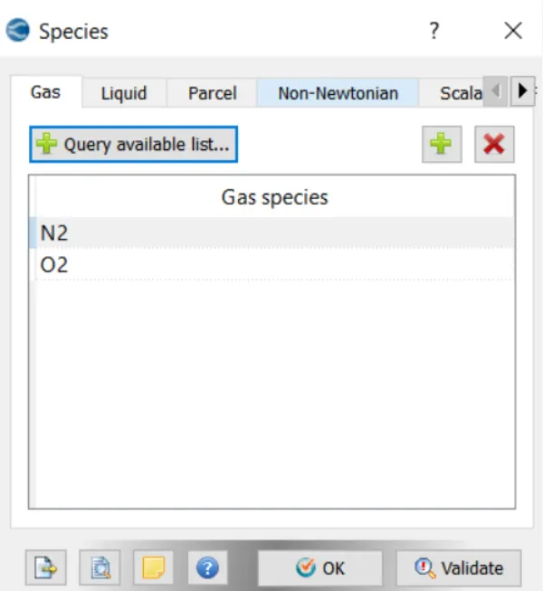
• Gas simulation is checked. The species are O2 and N2.

• Simulation Parameter -

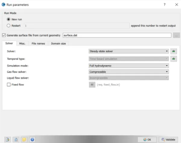
In Run Parameters- two main things to be considered

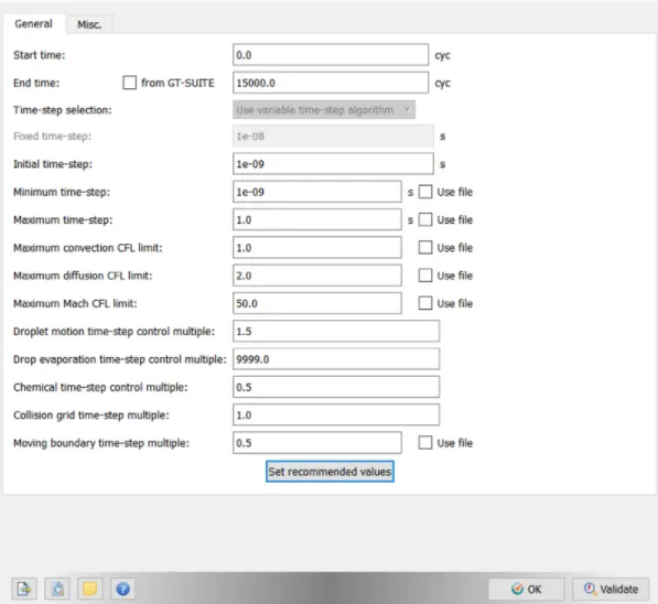
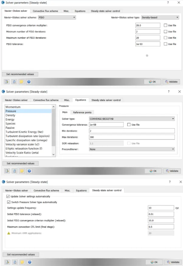
(a). Selected the following solver setting.

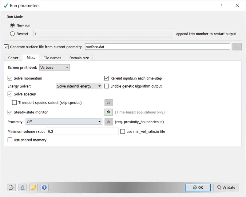
• Steady-State Monitor:

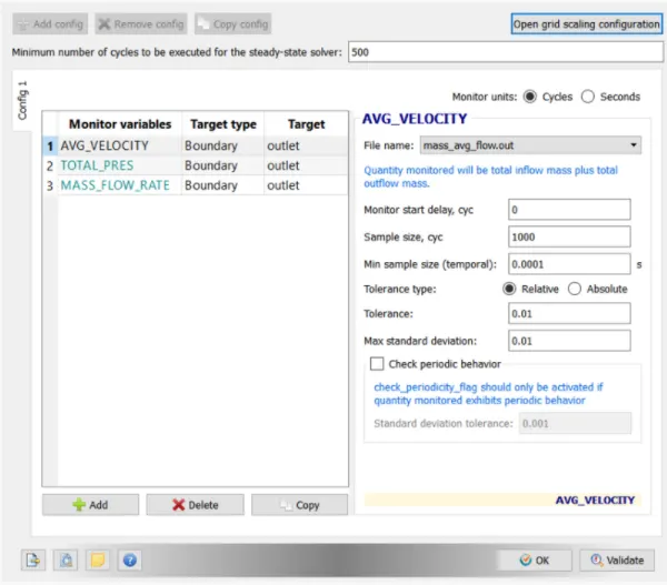
• Simulation Parameters:

• Solver Parameters[Steady-State]

• Boundary Conditions:

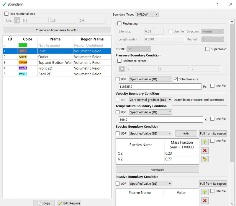
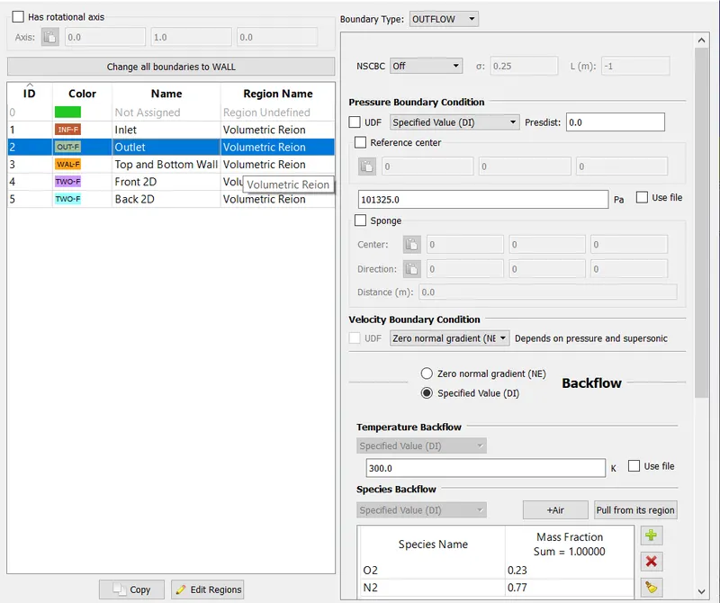
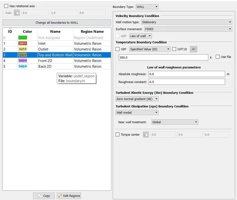
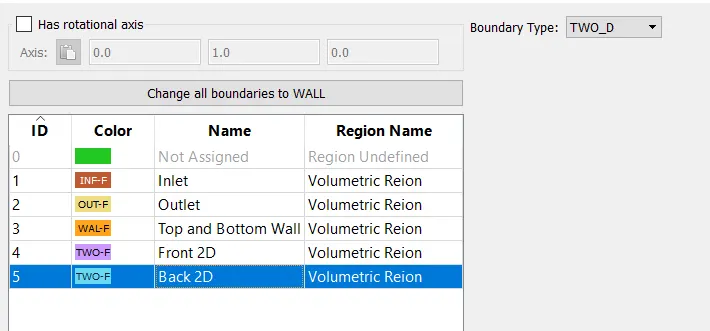
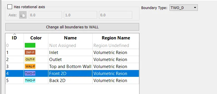
• Region and Initialization:

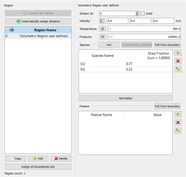
• Physical Models: Uncheck Turbulence Modeling in this Case.

• Grid Control:

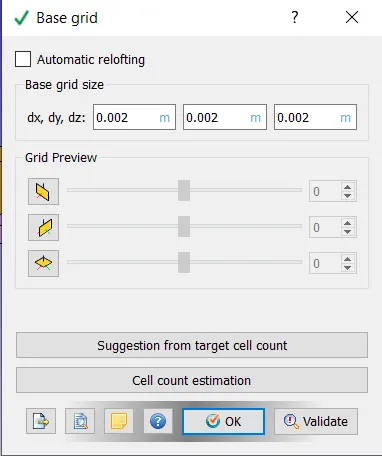
• Post Variable Selection:

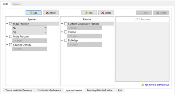
• Output Files:

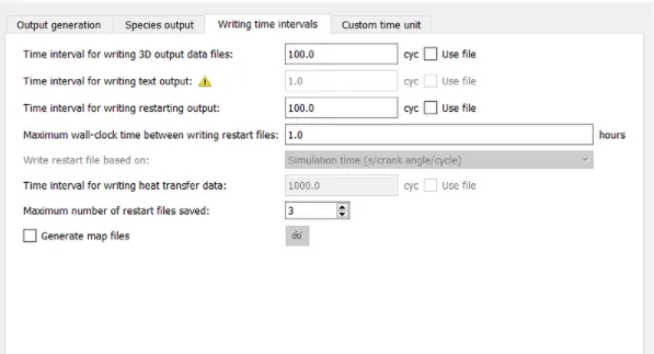
• Once the case setup is complete all the input files are exported to a specific folder.
• Then Cygwin is used to solve the inputs and once the simulation is complete converge converts the data into a format that can be read by pareview.
• Post-processing is done in Paraview.

lV. RESULTS

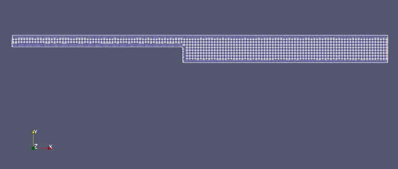
1. Grid Size = 2e-3 m

• Mesh

• Mass Flow Rate Plots

• Velocity Plots

• Pressure Plots

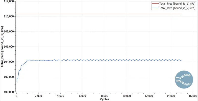
• Total Cell Count plots

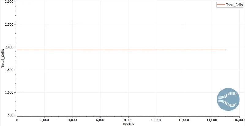
• Flow Separation

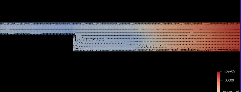
• Velocity Contours

• Pressure Contours

2. Grid Size = 1.5e-3 m

• Mesh

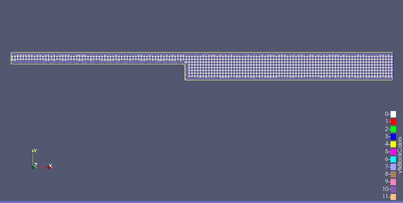
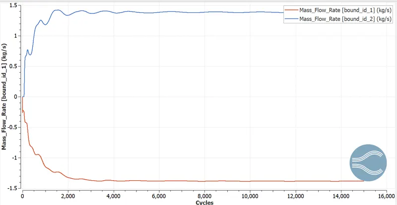
• Mass Flow Rate

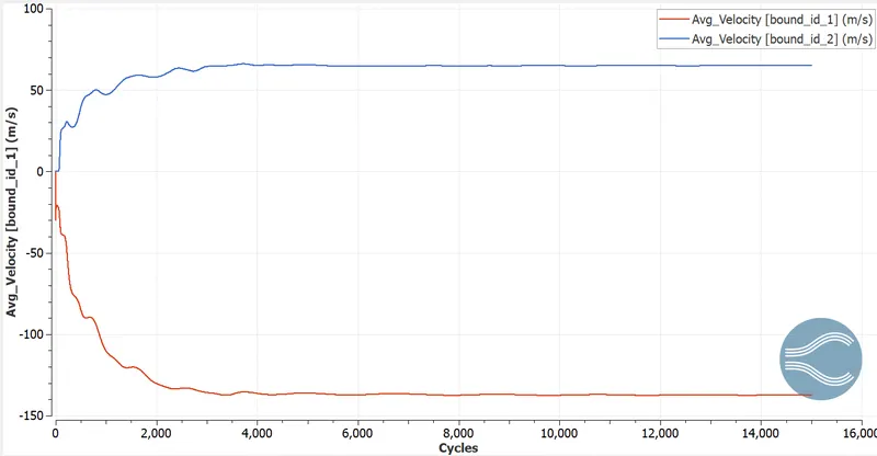
• Velocity Plots

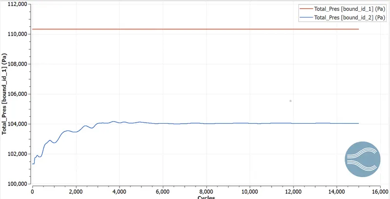
• Pressure Plots

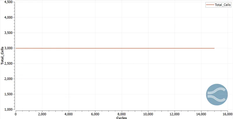
• Total Cell Count

• Flow Separation

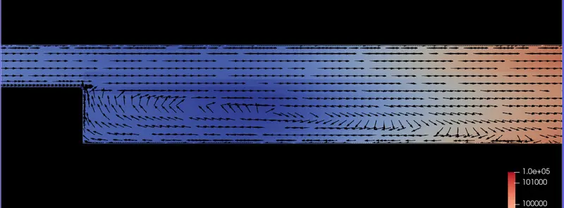
• Velocity Contours

• Pressure Contours

3. Grid Size =1.0e-3 m

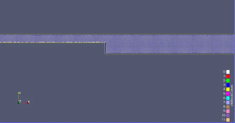
• Mesh

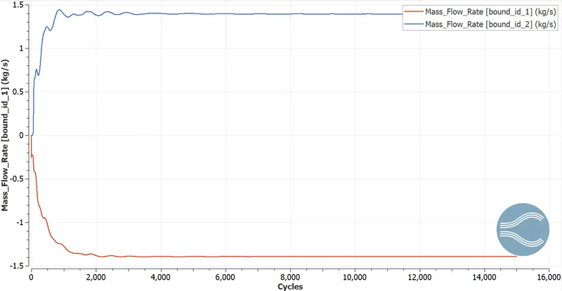
• Mass Flow Rate Plots

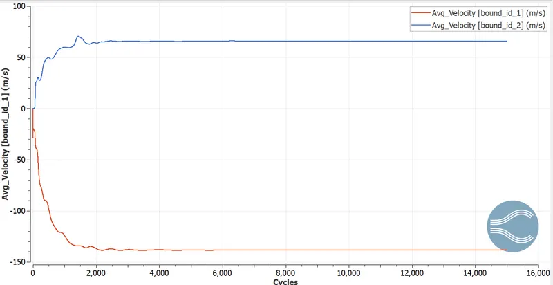
• Velocity Plot

• Pressure Plot

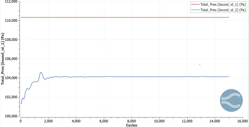
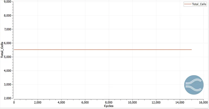
• Total Cell Count

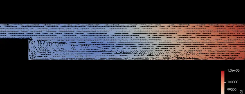
• Flow Separation

• Velocity Contour

• Pressure Contour

V. OBSERVATION

• From the simulations performed it is clear that for mesh size the total cell increases by refining the mesh. As the mesh becomes finer and finer the total cell count also increases, as the cell count increases the computational time also increases.
• From pressure contours, it is clear that pressure is constant at the outlet boundary but decreases in the inlet boundary.
• Pressure reduces at the inlet, due to excessive momentum loss near the step wall, The flow separation resulting in a zone with a pressure gradient is called the recirculation zone. The velocity vector plot clearly shows the recirculation zone in all the cases.
• Near the step in geometry, we can see the separation of the flow. This is due to the effect of boundary layer separation. Due to this, there is a disturbance in pressure and velocity. At this point, fluid separates and tends to recirculate.
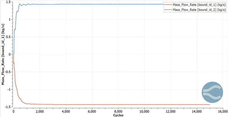
• The mass Flow Rate at the outlets for the refined cases is almost the same. When both inlets and outlets are compared we can observe a positive flow and a negative flow.
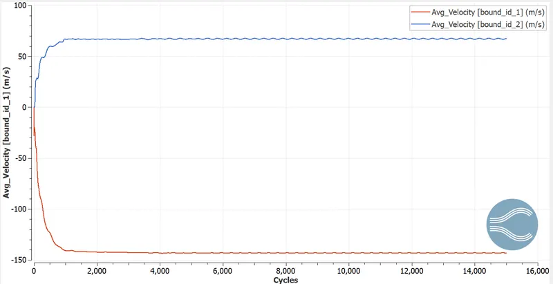
• Velocity in the initial case is highest but as the mesh is coarse it is generally not preferred to be accurate. In the next two cases, it is calculated more accurately.

Vl. FLOW SEPARATION

Near the step in geometry, we can see the separation, this is due to boundary layer separation. Due to the change in an area, there is a pressure drop, which leads to the separation of the flow. The boundary layer separation is a phenomenon that occurs when fluid experiences a sudden change in the area to the path of the flow.

Vll. CONCLUSION