Challenge

EVALUATION OF ADIABATIC FLAME TEMPERATURE USING PYTHON AND CANTERA

HHimanshu Chavan3 Jul 2021

EVALUATION OF ADIABATIC FLAME TEMPERATURE USING PYTHON AND CANTERA

l. OBJECTIVE

1. Write a program to analyze the effect of equivalence ratio on the final adiabatic temperature of methane contained in a constant volume chamber. Also, compare the result with those obtained using Cantera.

2.Write a program to analyze the effect of frictional heat loss on the final adiabatic temperature of methane contained in a constant pressure chamber.

3. Write a program to calculate the AFT of the combustion process for a given equivalence ratio and heat loss fraction.

4. Write a program to analyze the variation of Adiabatic Flame Temperature for different hydrocarbons (Ethane, Ethene & Ethyne) contained in a constant pressure chamber.

5.Write a program to analyze the variation of Adiabatic Flame Temperature for different alkenes (Methane, Ethane & Propane) contained in a constant pressure chamber.

ll. INTRODUCTION

A. Adiabatic Flame Temperature (AFT)

In a combustion process, the heat produced during the exothermic chemical reaction is released to their product and the temperature of the products is raised. There is no possibility for dissipation of the heat to the surroundings and the process will be adiabatic as there is no heat loss to the surrounding.

As a result, the temperature of the products suddenly increases and it produces a flame. This will heat the product gases in the flame region and the temperature rise will be maximum. This highest temperature is known as the adiabatic flame temperature.

B. Processes Involved In Combustion

There are two processes which can determine the final AFT of the system-

1. Constant Volume Process

The Internal Energy o reactants and the products are equal in a constant volume process.

`U_R =U_P`

`H_R-(PV)_R=H_P-(PV)_P`

`H_R-(nRT)_R=H_P-(nRT)_P`

`(H_P-H_R)-((nRT)_P-(nRT)_R)=0`

2. Constant Pressure Process

The enthalpy of reactants and products are equal in a constant pressure process.

`H_R=H_P`

`H_P-H_R=0`

C. Stoichiometric Equation

The general stoichiometric equation for the combustion of a hydrocarbon can be represented as follows-

`C_xH__y+ar(O_2+3.76N_2)rarrxCO_2+(y/2)H_2O+(3.76ar)N_2`

The term stoichiometric refers to the presence of just enough oxygen to completely burn all the fuel. The AFT obtained at the stoichiometric ratio is maximum.

However, such ideal conditions are rarely observeed in a combustion process and therefore there is always some additional species leftover at the end ofthe process.

D. Fuel- Air Equivalence Ratio(`phi`)

The fuel -air equivalence ratio is defined as the ratio of the Fuel- Air ratio to the corresponding stoichoimetric Fuel-Air ratio of the given combustion reaction.

`(Fuel//Air)_(Actual) /(Fuel//Air)_(St )`

as we can say

`phi`= 1 Stoichiometric Mixture

`phi` < 1 Fuel lean Mixture (excess air)

`phi` > 1 Fuel rich Mixture(excess fuel)

E. General Eqaution Of Combustion Process

The general form of a Stoichiometric Equation -

`C_xH_y+(x+y/4).(O_2+3.76.N_2)rarrx.CO_2+(y/2).H_2O+(x+y/4).N_2`

For Lean Mixture: A lean mixture of combustion of methane has an extra oxygen atom formed in the product side:-

`CH_4+(2/phi).(O_2+3.76.N_2)rarrCO_2+2H_O+((2/phi)-2)O_2+(7.53/phi).N_2`

For Rich Mixture: Similarly for a rich mixture CO(carbon monoxide) is formed.

`CH_4+(2/phi).(O_2+3.76.N_2) rarr((4/phi)-3)CO_2+2H_2O+(4-(4/phi))CO+(7.52/phi).N_2`

F. Enthalpy of the System

The enthalpy of the system depends on the species involved in the process and the temperature of the system. The enthalpy of the system can be calculated using the formula -

`H=(a1+a2T/2+a3T^2/3+a4T^3/4+a5T^4/5+(a6)/T).R.T`

where a1,a2,a3,a4,a5,a6 are the numerical coefficients supplied from NASA Thermodynamic Data File.

G. Newton - Raphson Method

It is a root-finding algorithm that produces successively better approximations to the roots of a real-valued function.

The general formula for Newton Raphson method can be given as-

`x_(n+1)=x_n-alphaf(x_n)/(f'(x_n))`

where

`f(x)rarr`Real-valued function

`f'(x)rarr`Derivative of the function

`alpha rarr`Multiplicity of the root

lll. PYTHON AND CANTERA PROGRAMS AND OUTPUTS

In this project, we shall be considering the following cases-

1. Efffect of equivalence ratio on the adiabatic falme temperature.

2. Effect of heat loss on the adiabatic flame temperature.

3. Calculation of AFT for a given equivalence ratio and heat loss fraction.

4. Variation of adiabatic flame temperature for different hydrocarbons.

5. Variation of Adiabatic flame temperature for different alkanes.

CASE 1 - EFFECT OF EQUIVALENCE RATIO ON ADIABATIC FLAME TEMPERATURE

1.Process: Combustion of hydrocarbon in a Constant Volume Chamber.

2. Hydrocarbon:

Methane: x=1; y=4

3. Code:

"""
General Equation:
	CxHy + (x+y/4)(O2 + 3.76N2) = x.Co2 + (y/2)H2o + 3.76(x+y/4)N2 
	x = 1; y = 4; 

Stoichiometric Equation (phi = 1):
	CH4 + 2(O2 + 3.76N2) = CO2 + 2H2O + 7.52N2
Lean Mixture Equation (phi < 1):
	CH4 + (2/phi)(O2 + 3.76N2) = CO2 + 2H2O + (7.52/phi)N2 + (2/phi-2)O2
Rich Mixture Equation (phi > 1):
	CH4 + (2/phi)(O2 + 3.76N2) = (4/phi-3)CO2 + 2H2O + (7.52/phi)N2 + (4 - 4/phi)CO

"""
import matplotlib.pyplot as plt
import math
import numpy as np

R = 8.314 # J/mol-k

# NASA Polynomail Constants
# Low temperature coefficient (Reactanats) at STP condition

ch4_coeffs_l =  [5.14987613E+00, -1.36709788E-02, 4.91800599E-05, -4.84743026E-08, 1.66693956E-11, -1.02466476E+04, -4.64130376E+00 ]
o2_coeffs_l  =  [3.78245636E+00, -2.99673416E-03, 9.84730201E-06, -9.68129509E-09, 3.24372837E-12, -1.06394356E+03,  3.65767573E+00 ]
n2_coeffs_l  =  [0.03298677E+02,  0.14082404E-02,-0.03963222E-04,  0.05641515E-07,-0.02444854E-10, -0.10208999E+04,  0.03950372E+02 ]

# High temperature coefficient (Product) 

n2_coeffs_h  =  [0.02926640E+02, 0.14879768E-02, -0.05684760E-05,  0.10097038E-09, -0.06753351E-13, -0.09227977E+04, 0.05980528E+02 ]
co2_coeffs_h =  [3.85746029E+00, 4.41437026E-03, -2.21481404E-06,  5.23490188E-10, -4.72084164E-14, -4.87591660E+04, 2.27163806E+00 ]
h20_coeffs_h =  [3.03399249E+00, 2.17691804E-03, -1.64072518E-07, -9.70419870E-11,  1.68200992E-14, -3.00042971E+04, 4.96677010E+00 ]
o2_coeffs_h  =  [3.28253784E+00, 1.48308754E-03, -7.57966669E-07,  2.09470555E-10, -2.16717794E-14, -1.08845772E+03, 5.45323129E+00 ]
co_coeffs_h  =  [2.71518561E+00, 2.06252743E-03, -9.98825771E-07,  2.30053008E-10, -2.03647716E-14, -1.41518724E+04, 7.81868772E+00 ]

# Function to evaluate Enthalpy

def h(T, co_effs):  

	a1 = co_effs[0]
	a2 = co_effs[1]
	a3 = co_effs[2]
	a4 = co_effs[3]
	a5 = co_effs[4]
	a6 = co_effs[5]

	return (a1 + a2*T/2 + a3*pow(T,2)/3 + a4*pow(T,3)/4 + a5*pow(T,4)/5 + a6/T)*R*T

# Function that represent the root finding problem		

def f(T, phi):

	# Products At temperature T

	h_co2_p = h(T, co2_coeffs_h)
	h_h2o_p = h(T, h20_coeffs_h)
	h_n2_p  = h(T, n2_coeffs_h)
	h_o2_p  = h(T, o2_coeffs_h)
	h_co_p  = h(T, co_coeffs_h)

	if phi >= 1 : # Conditional Loop based on equivalence Ratio enthalpy of product will be found out
		H_products = (4/phi-3)*h_co2_p + 2*h_h2o_p + (7.52/phi)*h_n2_p + (4-4/phi)*h_co_p
		N_products = ((4/phi - 3) + 2 + (7.52/phi) + (4-4/phi))*R*T
	elif phi < 1:
		H_products = h_co2_p + 2*h_h2o_p + (7.52/phi)*h_n2_p + (2/phi-2)*h_o2_p
		N_products = (1 + 2 + (7.52/phi) + (2/phi-2))*R*T

	
	# Reactants At Standard Temperature

	T_std = 298.15
	h_ch4_r = h(T_std, ch4_coeffs_l)
	h_o2_r =  h(T_std, o2_coeffs_l)
	h_n2_r =  h(T_std, n2_coeffs_l)

	H_reactants = h_ch4_r + (2/phi)*h_o2_r + (7.52/phi)*h_n2_r
	N_reactants = (1 + (2/phi) + (7.52/phi))*R*T_std

	if phi >= 1 : # Conditional Loop based on equivalence Ratio enthalpy of product will be found out
		H_products = (4/phi-3)*h_co2_p + 2*h_h2o_p + (7.52/phi)*h_n2_p + (4-4/phi)*h_co_p
		N_products = ((4/phi - 3) + 2 + (7.52/phi) + (4-4/phi))*R*T
	elif phi < 1:
		H_products = h_co2_p + 2*h_h2o_p + (7.52/phi)*h_n2_p + (2/phi-2)*h_o2_p
		N_products = (1 + 2 + (7.52/phi) + (2/phi-2))*R*T

	return (H_reactants - H_products) - (N_reactants - N_products)

	

# Function that represent the derivative of the root finding problem	


def fprime(T,phi):
	return (f(T+1e-6, phi ) - f(T,phi))/(1e-6)

# Using Newton-Raphson to solve iteratively
tol = 1e-3
alpha = 0.2
phi = [0.1, 0.2, 0.3, 0.4, 0.5, 0.6, 0.7, 0.8, 0.9, 1, 1.1, 1.2, 1.3, 1.4, 1.5, 1.6, 1.7, 1.8, 1.9, 2]
Temp_aft_py = [] # Defined arrays to store the values of temperature

for i in range(0,len(phi)):  # Loop to perform a root-finding procedure for all values of equivalence factor between 0.1 to 2
	T_guess = 1500
	while abs(f(T_guess, phi[i])) >= tol:
		T_guess = T_guess - alpha*((f(T_guess,phi[i]))/(fprime(T_guess,phi[i])))	# N-R iteration formula for getting better estimate of true roots
	Temp_aft_py.append(T_guess)	    
print(Temp_aft_py)
print()
 

# Cantera code - Exact Solution

import cantera as ct 
gas = ct.Solution('gri30.xml')

Temp_aft_ct = []

for i in range(0,len(phi)):
	
	n_total = 1+ (2/phi[i]) + (7.52/phi[i])
	n_ch4 = 1/n_total
	n_o2 = (2/phi[i])/n_total
	n_n2 = (7.52/phi[i])/n_total

	gas.TPX = 298.15, 101325, {'CH4':n_ch4, 'O2':n_o2, 'N2':n_n2}
	gas.equilibrate('UV', 'auto')
	Temp_aft_ct.append(gas.T)

print(Temp_aft_ct)

#Plotting Results
plt.plot(phi,Temp_aft_py,'-o',color='red',label='Python')
plt.plot(phi,Temp_aft_ct,'-o',color='blue',label='Cantera')	
plt.xlabel('Equivalence Ratio (phi)',fontsize=14)
plt.ylabel('Adiabatic Flame Temperature (K)',fontsize=14)
plt.xticks(np.arange(0, 2.1, step=0.2))
plt.yticks(np.arange(600, 3000, step=200))
plt.grid('on')

plt.legend(fontsize=14)
plt.show()

4. RESULT TABLE:

The results from the above program are shown below

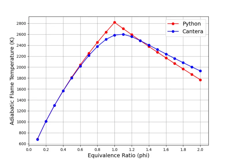
`phi` Python AFT [K] Cantera AFT [K]

0.1 681.68 679.62

0.2 1009.55 1009.43

0.3 1301.87 1300.75

0.4 1567.86 1563.56

0.5 1812.87 1802.09

0.6 2040.41 2018.37

0.7 2252.98 2211.72

0.8 2452.45 2377.51

0.9 2640.34 2506.67

1.0 2817.83 2585.88

1.1 2704.16 2600.54

1.2 2592.95 2556.49

1.3 2484.00 2484.06

1.4 2377.13 2403.26

1.5 2272.14 2321.03

1.6 2168.85 2239.55

1.7 2067.07 2159.52

1.8 1966.59 2081.14

1.9 1867.22 2004.48

2.0 1768.75 1929.53

5. OUTPUT:

AFT vs Equivalence Ratio for Methane-Air Combustion

6. RESULTS:

The AFT obtained from Python and Cantera is almost equal at an equivalence Ratio Lower than 0.8. This is because enough oxygen is present in the system to burn all the fuel into its corresponding products. These products have negligible additional species and hence, the results are almost equal for both Python and Cantera.

At an equivalence ratio greater than 1, the AFT curve obatined from Python deviates from the Cantera's Curve, beacuse the combustion process at these ratios results in the formation of additional minor species which are not considered by us in the Python program.

CASE 2- EFFECT OF HEAT LOSS ON ADIABATIC FLAME TEMPERATURE

1. Process:

Combustion of hydrocarbon in a Constant Pressure Chamber
Equivalence Ratio, `phi`= 1
Due to heat loss, the reaction is no longer adiabatic and hence, we will refer tp AFT as just FT (flame temperature)
The Heat loss from the reaction is programmed as a factor(H_loss) of the maximum possible heat loss from the reaction.
The maximum possible heat loss from the reaction is calculated as the lower heating value(LHV) of the reaction. LHV is calculated from the difference in the enthalpies of reactants and products when both are considered at STP. Since N2 from both the reactants and the products side is considered at `T_(std)=`298.15 K, it will cancel each other and can effectively be neglected from the calculation altogether as `LHV=H_(CH4)^298.15+2H_(O_2)^298.15-H_(CO_2)^298.15-2H_(H_2O)^298.15`
The heat loss factor(H_loss) is varied from 0 (no heat loss) to 1 (all heat loss) as a multiplier of the LHV.
Since the heat is lost from the reaction, lesser heat is available for the products to form and the equilibrium condition (root-finding function) for this reaction is: `H_(PRODUCTS)-H_(REACTANTS)+H_(LOSS)=0`

2. Hydrocarbon:

Methane: x = 1; y = 4

3. Code:

"""
General Equation:
	CxHy + (x+y/4)(O2 + 3.76N2) = x.Co2 + (y/2)H2o + (x+y/4)*3.76*N2 
	x = 1; y = 4; 

Stoichiometric Equation (phi = 1):
	CH4 + 2(O2 + 3.76N2) = CO2 + 2H2O + 7.52N2
Lean Mixture Equation (phi < 1):
	CH4 + (2/phi)(O2 + 3.76N2) = CO2 + 2H2O + (7.52/phi)N2 + (2/phi-2)O2
Rich Mixture Equation (phi > 1):
	CH4 + (2/phi)(O2 + 3.76N2) = (4/phi-3)CO2 + 2H2O + (7.52/phi)N2 + (4 - 4/phi)CO

"""

import matplotlib.pyplot as plt
import math
import numpy as np

R = 8.314 # J/mol-k


# NASA Polynomial Constants
# Low temperature coefficient (Reactanats) at STP condition

ch4_coeffs_l =  [5.14987613E+00, -1.36709788E-02, 4.91800599E-05, -4.84743026E-08, 1.66693956E-11, -1.02466476E+04, -4.64130376E+00 ]
o2_coeffs_l  =  [3.78245636E+00, -2.99673416E-03, 9.84730201E-06, -9.68129509E-09, 3.24372837E-12, -1.06394356E+03,  3.65767573E+00 ]
n2_coeffs_l  =  [0.03298677E+02,  0.14082404E-02,-0.03963222E-04,  0.05641515E-07,-0.02444854E-10, -0.10208999E+04,  0.03950372E+02 ]

# High temperature coefficient (Product) 

n2_coeffs_h  =  [0.02926640E+02, 0.14879768E-02, -0.05684760E-05,  0.10097038E-09, -0.06753351E-13, -0.09227977E+04, 0.05980528E+02 ]
co2_coeffs_h =  [3.85746029E+00, 4.41437026E-03, -2.21481404E-06,  5.23490188E-10, -4.72084164E-14, -4.87591660E+04, 2.27163806E+00 ]
h20_coeffs_h =  [3.03399249E+00, 2.17691804E-03, -1.64072518E-07, -9.70419870E-11,  1.68200992E-14, -3.00042971E+04, 4.96677010E+00 ]


# Function to evaluate Enthalpy

def h(T, coeffs):  

	a1 = coeffs[0]
	a2 = coeffs[1]
	a3 = coeffs[2]
	a4 = coeffs[3]
	a5 = coeffs[4]
	a6 = coeffs[5]

	return (a1 + a2*T/2 + a3*pow(T,2)/3 + a4*pow(T,3)/4 + a5*pow(T,4)/5 + a6/T)*R*T

# Function that represent the root finding problem		

def f(T, H_loss):

	# Products At temperature T

	h_co2_p = h(T, co2_coeffs_h)
	h_h2o_p = h(T, h20_coeffs_h)
	h_n2_p  = h(T, n2_coeffs_h)
	    
	H_products = h_co2_p + 2*h_h2o_p + 7.52*h_n2_p 

    # Reactants At Standard Temperature

	T_std   = 298.15
	h_ch4_r = h(T_std, ch4_coeffs_l)
	h_o2_r  = h(T_std, o2_coeffs_l)
	h_n2_r  = h(T_std, n2_coeffs_l)

	H_reactants = h_ch4_r + 2*h_o2_r + 7.52*h_n2_r

	
	# Lower Heating Value

	LHV = h(T_std, ch4_coeffs_l) + 2*h(T_std, o2_coeffs_l) - h(T_std,co2_coeffs_h) - 2*h(T_std,h20_coeffs_h)
	return H_products - H_reactants + (H_loss * LHV)



# Function that represent the derivative of the root finding problem	


def fprime(T,H_loss):
	return (f(T+1e-6, H_loss) - f(T, H_loss)) /(1e-6)


# Using Newton-Raphson to solve iteratively
tol = 1e-3
alpha = 0.9
H_loss = np.arange(0, 1.05, step=0.05)
Temp_aft_py = [] # Defined arrays to store the values of temperature

for i in range(0,len(H_loss)):  # Loop to perform a root-finding procedure for all values of equivalence factor between 0 to 1.05
	T_guess = 1500
	while abs(f(T_guess,H_loss[i])) >= tol:
		T_guess = T_guess - alpha*((f(T_guess,H_loss[i]))/(fprime(T_guess,H_loss[i])))	# N-R iteration formula for getting better estimate of true roots
	Temp_aft_py.append(T_guess)	    

   	
print(Temp_aft_py[7])
 

#Plotting Results
plt.plot(H_loss,Temp_aft_py,'-o',color='red')
plt.plot(H_loss[7],Temp_aft_py[7],'-o',color='black',label='H_loss = 0.35')	
plt.xlabel('Heat Loss Ratio',fontsize=14)
plt.ylabel('Adiabatic Flame Temperature (K)',fontsize=14)
plt.xticks(np.arange(0, 1.05, step=0.1))
plt.yticks(np.arange(250, 2500 , step=250))
plt.grid('on')
plt.title('AFT VS Heat Loss Ratio For Metahne-Air Combustion', fontsize=16, fontweight='bold')
plt.legend(fontsize=14)
plt.show()

4. OUTPUT:

5. RESULTS

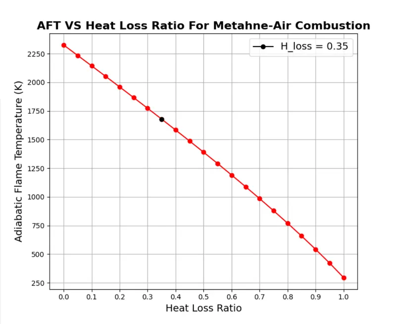
It can be clearly seen that as the heat loss from the reaction increases, the flame temperature of the products consistently reduces as less heat is available for the reaction.
At H_loss = 0, no heat is lost from the reaction and hence FT = AFT = 2325.6 K.
At H_loss = 1, all the heat is lost from the reaction and no heat is left for the products to form, hence the flame temperature is `T_(STD)=`298.15 K.
From the graph, the flame temperature of methane combustion with H_loss = 0.35 is calculated as 1678.81 K

CASE 3- VARIATION OF AFT FOR DIFFERENT HYDROCARBON

1. Process:

Combustion of hydrocarbon in a constant Pressure Chamber
Equivalence Ratio, `phi =1`

2. Hydrocarbon:

Ethane: `C_2H_6+3.5(O_2+3.76N_2)rarr2CO_2+3H_2O+13.16N_2`
Ethene: `C_H_4+3(O_2+3.76N_2)rarr2CO_2+2H_2O+11.28N_2`
Ethyne: `C_2H_2+2.5(O_2+3.76N_2)rarr2CO_2+H_2O+9.4N_2`

3. Code:

"""
General Hydrocarbon Equation:
	CxHy + (x+y/4)(O2 + 3.76N2) = x.Co2 + (y/2)H2o + 3.76(x+y/4)N2 
"""

import matplotlib.pyplot as plt
import math
import numpy as np
import cantera as ct

R = 8.314 # J/mol-k
T_std = 298.15
#Function to evaluate Enthalpy

def h(T, coeffs):  

	a1 = coeffs[0]
	a2 = coeffs[1]
	a3 = coeffs[2]
	a4 = coeffs[3]
	a5 = coeffs[4]
	a6 = coeffs[5]

	return (a1 + a2*T/2 + a3*pow(T,2)/3 + a4*pow(T,3)/4 + a5*pow(T,4)/5 + a6/T)*R*T

# NASA Polynomial Constants
# Low temperature coefficient (Reactanats) at STP condition

c2h6_coeffs_l =  [4.29142492E+00, -5.50154270E-03, 5.99438288E-05, -7.08466285E-08, 2.68685771E-11, -1.15222055E+04,  2.66682316E+00 ]
c2h4_coeffs_l =  [3.95920148E+00, -7.57052247E-03, 5.70990292E-05, -6.91588753E-08, 2.69884373E-11,  5.08977593E+03,  4.09733096E+00 ]
c2h2_coeffs_l =  [8.08681094E-01,  2.33615629E-02,-3.55171815E-05,  2.80152437E-08,-8.50072974E-12,  2.64289807E+04,  1.39397051E+01 ]
o2_coeffs_l   =  [3.78245636E+00, -2.99673416E-03, 9.84730201E-06, -9.68129509E-09, 3.24372837E-12, -1.06394356E+03,  3.65767573E+00 ]
n2_coeffs_l   =  [0.03298677E+02,  0.14082404E-02,-0.03963222E-04,  0.05641515E-07,-0.02444854E-10, -0.10208999E+04,  0.03950372E+02 ]

# High temperature coefficient (Product) 

n2_coeffs_h  =  [0.02926640E+02, 0.14879768E-02, -0.05684760E-05,  0.10097038E-09, -0.06753351E-13, -0.09227977E+04, 0.05980528E+02 ]
co2_coeffs_h =  [3.85746029E+00, 4.41437026E-03, -2.21481404E-06,  5.23490188E-10, -4.72084164E-14, -4.87591660E+04, 2.27163806E+00 ]
h20_coeffs_h =  [3.03399249E+00, 2.17691804E-03, -1.64072518E-07, -9.70419870E-11,  1.68200992E-14, -3.00042971E+04, 4.96677010E+00 ]


# Function that represent the root finding problem		


def f(T, ntype):

	# Products At temperature T

	h_co2_p = h(T, co2_coeffs_h)
	h_h2o_p = h(T, h20_coeffs_h)
	h_n2_p  = h(T, n2_coeffs_h)

	    
	# Reactants At Standard Temperature

	h_c2h6_r = h(T_std, c2h6_coeffs_l)
	h_c2h4_r = h(T_std, c2h4_coeffs_l)
	h_c2h2_r = h(T_std, c2h2_coeffs_l)	
	h_o2_r  = h(T_std, o2_coeffs_l)
	h_n2_r  = h(T_std, n2_coeffs_l)

	if ntype==1:
		x = 2
		y = 6
		h_fuel = h_c2h6_r
		
	elif ntype==2:
		x = 2
		y = 4
		h_fuel = h_c2h4_r
	elif ntype==3:
		x = 2
		y = 2
		h_fuel = h_c2h2_r

	H_reactants = h_fuel + (x+y/4)*h_o2_r + 3.76*(x+y/4)*h_n2_r
	H_products  = x*h_co2_p + (y/2)*h_h2o_p + 3.76*(x+y/4)*h_n2_p

	return (H_products - H_reactants)

# Defining the derivative of the function
def fprime(T, ntype):
	return (f(T+1e-6, ntype) - f(T, ntype))/(1e-6)

#Newton-Rapson Solver	
alpha = 1
tol = 1e-3	
ntype = [1, 2, 3]
T_aft_py = []

for i in range(0, len(ntype)):
	T_guess = 1500 # k
	while abs(f(T_guess, ntype[i] )) >= tol:
		T_guess = T_guess - alpha*((f(T_guess, ntype[i]))/(fprime(T_guess, ntype[i])))
	T_aft_py.append(T_guess)
print(T_aft_py)
print()

#Plotting the Results
plt.bar(['Ethane ( C_2H_6)', 'Ethene (C_2H_4)', 'Ethyne (C_2H_2)'], T_aft_py)
plt.ylabel('Adiabatic Flame Temperature [K]', fontsize=12)
plt.title('AFT VS Type Of Hydrocarbon (Python)', fontsize=13,fontweight='bold')
plt.show()			

"""
Solution Obtained by cantera
"""
gas = ct.Solution('gri30.xml')
T_aft_ct = []

for i in range(0, len(ntype)):

	if ntype[i]==1:
		x = 2
		y = 6
		fuel = 'C2H6'		
	elif ntype[i]==2:
		x = 2
		y = 4
		fuel = 'C2H4'
	elif ntype[i]==3:
		x = 2
		y = 2
		fuel = 'C2H2'
	n_tot = 1 + (x+y/4) + 3.76*(x+y/4)
	n_fuel = 1/n_tot
	n_o2 = (x+y/4)/n_tot
	n_n2 = (3.76*(x+y/4))/n_tot

	# Defining the gas mixture
	gas.TPX = 298.15, 101325, {fuel:n_fuel, 'O2': n_o2, 'N2': n_n2}

	# Calculating the equilibrium conditions
	gas.equilibrate('HP','auto')
	T_aft_ct.append(gas.T)
print(T_aft_ct)	


# Plotting The cantera results
plt.bar(['Ethane (C_2H_6)', 'Ethene (C_2H_4)','Ethyne (C_2H_2)'], T_aft_py)
plt.ylabel('Adiabatic Flame Temperature [K]', fontsize= 12)
plt.title('AFT vs Type Of Hydrocarbon (Cantera)',fontsize=13,fontweight='bold')
plt.show()

4. OUTPUTS:

5. RESULTS

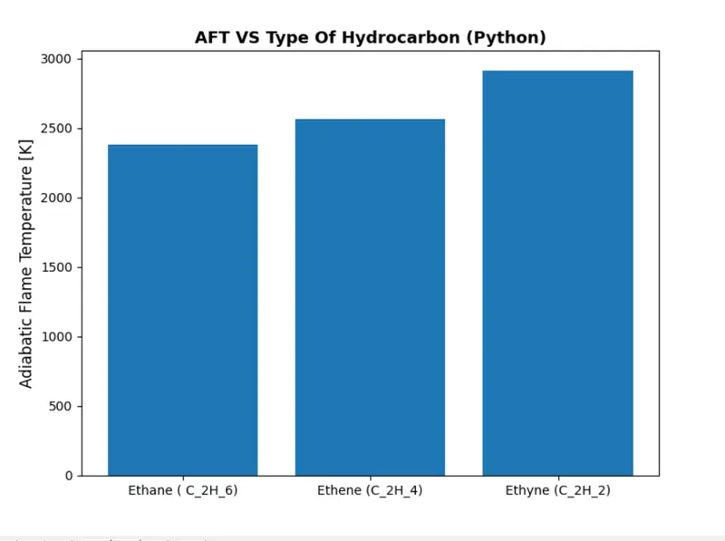
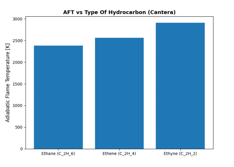
FUEL Python AFT [K] Cantera [K]

Ethane 2379.85 2258.74

Ethene 2564.53 2368.64

Ethyne 2909.35 2539.67

We can see that the AFT increases considerably for ethene and ethyne campared to ethane becaues of their multiple C-atom bonds. For multiple C-atom bonds, more energy is required to break the bond and cause the reaction, and hence higher temperatures are generated. Also, we can see that the difference in the solution obtained from Python and Cantera differs by more amount as the hydrocarbon becomes more complex. This is because the combustion reaction of ethene and ethyne can produce more additional products than anticipated.

CASE 4 - VARIATION OF ADIABATIC FLAME TEMPERATURE FOR DIFFERENT ALKANES

1. Process

Combustion of hydrocarbon in a Constant Pressure Chamber.
Equivalence Ratio, `phi=1`
Heat Loss Fraction = 0

2. Hydrocarbon:

Methane: x=1; y=4
Ethane: x=2; y=6
Propane: x=3; y=8

3. CODE:

"""
General Hydrocarbon Equation:
	CxHy + (x+y/4)(O2 + 3.76N2) = x.Co2 + (y/2)H2o + 3.76(x+y/4)N2 

	Methane: CH4 + 2(O2 + 3.76N2) <=> CO2 + 2H2O + 7.52N2
	Ethane: C2H6 + 3.5(O2 +3.76N2) <=> 2CO2 + 3H2O +13.16N2
	Propane: C3H8 + 5(O2 + 3.76N2) <=> 3CO2 + 4H2O + 18.8N2
"""

import matplotlib.pyplot as plt
import math
import numpy as np
import cantera as ct

R = 8.314 # J/mol-k
T_std = 298.15
#Function to evaluate Enthalpy

def h(T, coeffs):  

	a1 = coeffs[0]
	a2 = coeffs[1]
	a3 = coeffs[2]
	a4 = coeffs[3]
	a5 = coeffs[4]
	a6 = coeffs[5]

	return (a1 + a2*T/2 + a3*pow(T,2)/3 + a4*pow(T,3)/4 + a5*pow(T,4)/5 + a6/T)*R*T

# NASA Polynomial Constants
# Low temperature coefficient (Reactanats) at STP condition
ch4_coeffs_l  =  [5.14987613E+00, -1.36709788E-02, 4.91800599E-05, -4.84743026E-08, 1.66693956E-11, -1.02466476E+04, -4.64130376E+00 ]
c2h6_coeffs_l =  [4.29142492E+00, -5.50154270E-03, 5.99438288E-05, -7.08466285E-08, 2.68685771E-11, -1.15222055E+04,  2.66682316E+00 ]
c3h8_coeffs_l =  [0.93355381E+00,  0.26424579E-01, 0.61059727E-05, -0.21977499E-07, 0.95149253E-11, -0.13958520E+05,  0.19201691E+02 ]
o2_coeffs_l   =  [3.78245636E+00, -2.99673416E-03, 9.84730201E-06, -9.68129509E-09, 3.24372837E-12, -1.06394356E+03,  3.65767573E+00 ]
n2_coeffs_l   =  [0.03298677E+02,  0.14082404E-02,-0.03963222E-04,  0.05641515E-07,-0.02444854E-10, -0.10208999E+04,  0.03950372E+02 ]

# High temperature coefficient (Product) 

n2_coeffs_h  =  [0.02926640E+02, 0.14879768E-02, -0.05684760E-05,  0.10097038E-09, -0.06753351E-13, -0.09227977E+04, 0.05980528E+02 ]
co2_coeffs_h =  [3.85746029E+00, 4.41437026E-03, -2.21481404E-06,  5.23490188E-10, -4.72084164E-14, -4.87591660E+04, 2.27163806E+00 ]
h20_coeffs_h =  [3.03399249E+00, 2.17691804E-03, -1.64072518E-07, -9.70419870E-11,  1.68200992E-14, -3.00042971E+04, 4.96677010E+00 ]


# Function that represent the root finding problem		


def f(T, ntype):

	# Products At temperature T

	h_co2_p = h(T, co2_coeffs_h)
	h_h2o_p = h(T, h20_coeffs_h)
	h_n2_p  = h(T, n2_coeffs_h)

	    
	# Reactants At Standard Temperature

	h_ch4_r =  h(T_std, ch4_coeffs_l)
	h_c2h6_r = h(T_std, c2h6_coeffs_l)
	h_c3h8_r = h(T_std, c3h8_coeffs_l)	
	h_o2_r  = h(T_std, o2_coeffs_l)
	h_n2_r  = h(T_std, n2_coeffs_l)

	if ntype==1:
		x = 1
		y = 4
		h_fuel = h_ch4_r
		
	elif ntype==2:
		x = 2
		y = 6
		h_fuel = h_c2h6_r
	elif ntype==3:
		x = 3
		y = 8
		h_fuel = h_c3h8_r

	H_reactants = h_fuel + (x+y/4)*h_o2_r + 3.76*(x+y/4)*h_n2_r
	H_products  = x*h_co2_p + (y/2)*h_h2o_p + 3.76*(x+y/4)*h_n2_p

	return (H_products - H_reactants)

# Defining the derivative of the function
def fprime(T, ntype):
	return (f(T+1e-6, ntype) - f(T, ntype))/(1e-6)

#Newton-Rapson Solver	
alpha = 1
tol = 1e-3	
ntype = [1, 2, 3]
T_aft_py = []

for i in range(0, len(ntype)):
	T_guess = 1500 # k
	while abs(f(T_guess, ntype[i] )) >= tol:
		T_guess = T_guess - alpha*((f(T_guess, ntype[i]))/(fprime(T_guess, ntype[i])))
	T_aft_py.append(T_guess)
print(T_aft_py)
print()

#Plotting the Results
plt.bar(['Methane ( CH_4)', 'Ethane (C_2H_6)', 'Propane (C_3H_8)'], T_aft_py)
plt.ylabel('Adiabatic Flame Temperature [K]', fontsize=12)
plt.title('AFT VS Type Of Hydrocarbon (Python)', fontsize=13,fontweight='bold')
plt.show()			

"""
Solution Obtained by cantera
"""
gas = ct.Solution('gri30.xml')
T_aft_ct = []

for i in range(0, len(ntype)):

	if ntype[i]==1:
		x = 1
		y = 4
		fuel = 'Ch4'		
	elif ntype[i]==2:
		x = 2
		y = 6
		fuel = 'C2H6'
	elif ntype[i]==3:
		x = 3
		y = 8
		fuel = 'C3H8'
	n_tot = 1 + (x+y/4) + 3.76*(x+y/4)
	n_fuel = 1/n_tot
	n_o2 = (x+y/4)/n_tot
	n_n2 = (3.76*(x+y/4))/n_tot

	# Defining the gas mixture
	gas.TPX = 298.15, 101325, {fuel:n_fuel, 'O2': n_o2, 'N2': n_n2}

	# Calculating the equilibrium conditions
	gas.equilibrate('HP','auto')
	T_aft_ct.append(gas.T)
print(T_aft_ct)	


# Plotting The cantera results
plt.bar(['Methane (CH_4)', 'Ethane (C_2H_6)','Propane (C_3H_8)'], T_aft_py)
plt.ylabel('Adiabatic Flame Temperature [K]', fontsize= 12)
plt.title('AFT vs Type Of Hydrocarbon (Cantera)',fontsize=13,fontweight='bold')
plt.show()

4. OUTPUT:

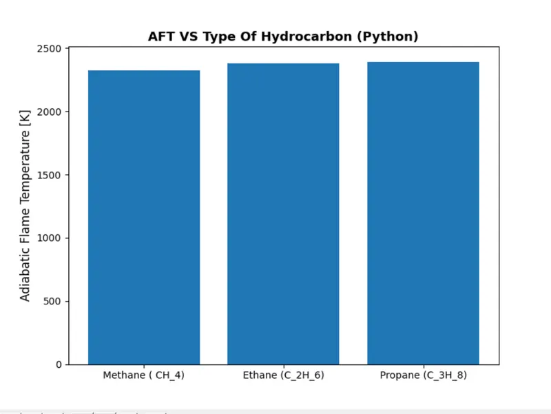
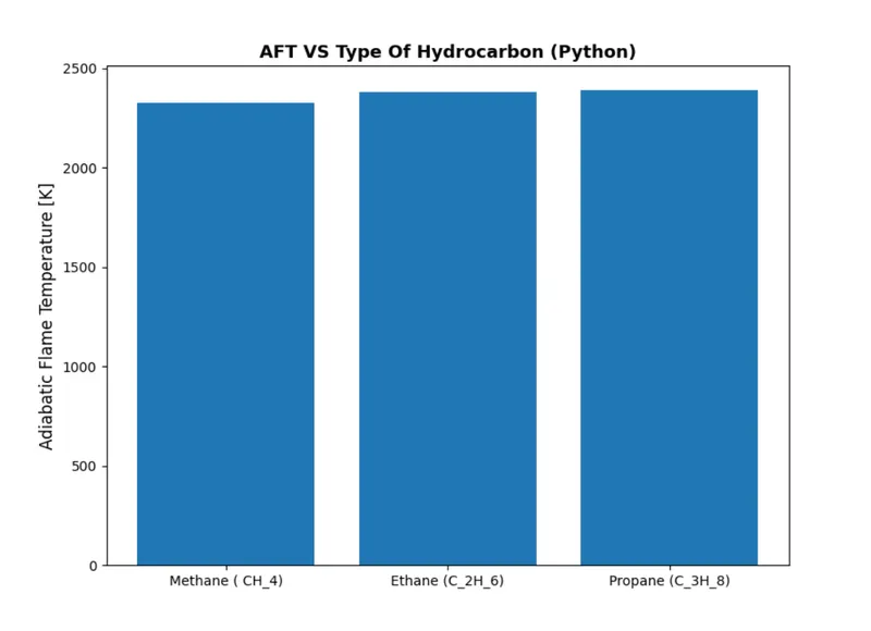
5. RESULTS:

FUEL PYTHON AFT [K] CANTERA AFT [K]

Methane 2325.6 2224.62

Ethane 2379.85 2258.74

Propane 2392.09 2265.70

We can see that the AFT does not vary much (`Delta<100K`) with a consequent increase in thr number of C-atom chains in a hydrocarbon. Also, in this case, the difference between the solution obtained from Python and Cantera does not differ by a huge amount.The reaction mechanism for alkanes is fairly simple and it does not produce any unanticipated products as opposed to the previous casewith combustion of alkenes and alkynes.

lV. CONCLUSIONS

The effect of equivalence ratio and fractional heat loss on a combustion reaction under different conditions is observed. Also, the variation of AFT for different types of hydrocarbons is determined.

EVALUATION OF ADIABATIC FLAME TEMPERATURE USING PYTHON AND CANTERA

Ship work like this
in your own course.

Talk to a career counsellor

Ship work like thisin your own course.

Talk to a career counsellor

Ship work like this
in your own course.