External flow simulation over an Ahmed body.

SIMULATION & ANALYSIS OF FLUID FLOW OVER AHMED BODY IN A WIND TUNNEL

l. OBJECTIVES

1. Simulate and analyze the flow of fluid over Ahmed Body in a wind tunnel.

2. Perform grid dependency test on the given setup.

3. Plot and analyze the velocity and pressure contours using a midplane along the direction of flow.

ll. INTRODUCTION

1. Ahmed Body

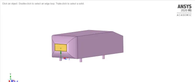
The Ahmed body is a bluff body or rather a generic car body (simplified vehicle model). The airflow around the Ahmed body captures the essential flow feature around an automobile and was first defined and characterized in the experimental work of Ahmed. Although it has a very simple shape, relevant to bodies in the automobile industry. This model is also used to describe the turbulent flow field around a car-like geometry. Once the numerical model is validated, it is used to design the new models of the car.

The Ahmed body is a geometric shape first proposed by S.R. Ahmed and Ramm in their research, '' Some Salient Features of the Time Averaged Ground Vehicle Wake'' in 1984. The purpose behind the design of this Ahmed Body is to study geometry's effect on the wakes of the ground vehicles.

2. Significance Of Ahmed Body

1. One of the reasons for Studying such a simplified car body is to understand the flow processes involved in drag production. By understanding the mechanisms involved in generating drag, One should be able to design a car to minimize drag and therefore minimize fuel consumption and maximize performance.

2. Several different types of experiments have also been performed on an actual model of Ahmed's body and hence there is a huge amount of experimental data available.

3. Negative pressure at Wake region and Point of Separation.

The flow around Ahmed's body is complicated. Due to the slant in the rear of the vehicle, flow separation and contour rotating vortices are generated at the slant edges. The drag force of Ahmed's Body reaches a maximum when the slant angle is 30 degrees.

For the Slant angle higher than this value, the adverse pressure gradient in between the slant and the roof is so intense that the flow fully detaches over the slant. Below these critical slant angles(30 degrees), the flow still separates but the pressure difference between the slant region and the side walls is still sturdy enough to generate substantial stream-wise vortices at the lateral slant edges. These prompt a downward motion over the slant, mainly in the downstream part. As a result, the flow separates at the upstream end of the slant can be coupled further to the downstream. The flow around the Ahmed Body has several flow separations from the front to the rear of the vehicle. The flow recirculation caused by these flow detachments contributes to the vehicle's drag. The Location point at which the flow separates determines the size of the separation zone, and accordingly the drag force, thus an exact simulation of the wake flow and the separation process is essential for the accurate result of drag predictions.

3. Y plus Value:

The Y+ value is a non-dimensional distance (based on local cell fluid velocity) from the wall to the first mesh node, as shown below figure. To use a wall function approach for a particular turbulence model with confidence, we need to ensure that our y+ values are within a certain range.

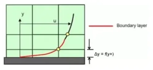
Considering the above figure it's important to ensure Y+ values are not so large that the first node falls outside the boundary layer region. If this happens, then the wall functions used by the turbulence model may incorrectly calculate the flow properties at this first calculation point which will introduce errors into pressure drop and velocity results.

Reynolds number, Re = `(rho VL)/mu`

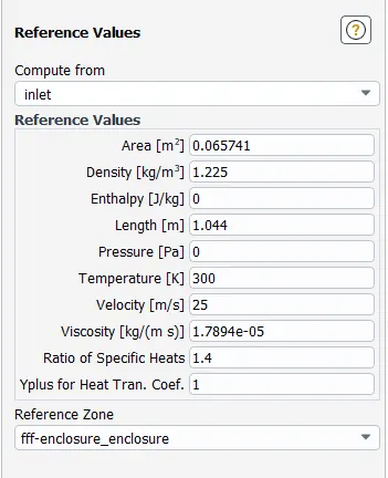
As we know inlet velocity V= 25m/s and material is air with density 1.225

`Re = (1.225xx25xx1.044)/(1.7894xx10^-5)`

`:. Re = 1786772.10`

`Cf =(0.0576)/((Re)^(1/5)`=0.00326

`Tomega = (Cfxxrhoxxv^2)/2`

`:.Tomega=(0.00326xx1.225xx25^2)/2`

`:.Tomega =1.24796N/(m^2)`

`u_f = sqrt((Tomega)/(rho)``:. u_f=sqrt(1.24796/1.225) = 1.009327m/s`

as we consider y+ value 5

hence first layer thickness,

`y1=(vy^+)/(rhou_f)`

`y1=(1.7894xx10^-5xx5)/(1.225xx1.009327)`

`y1=0.0716483`

Vl. INITIAL TEST - BASELIINE MESH

A. SPCECLAIM GEOMETRY

1.Ahmed Body

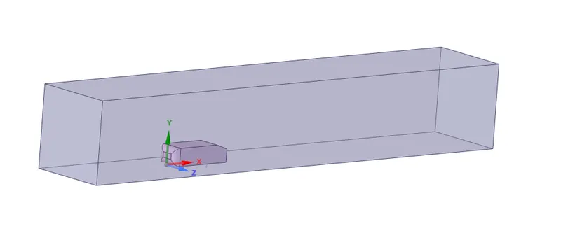
2. Ahmed Body In wind Tunnel

2.1 Model

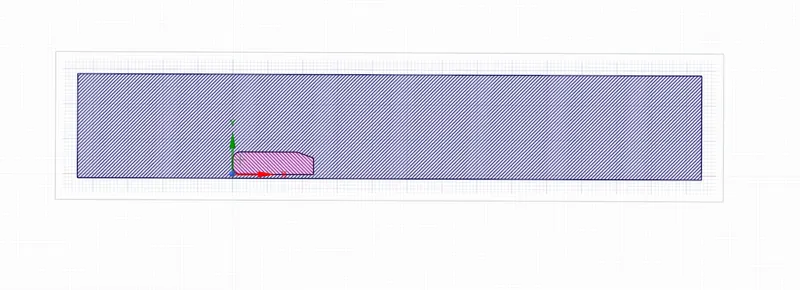
2.2 Section Plane

B. MESH

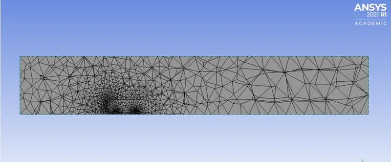
A basic mesh is generated using the standard values recommended by Ansys. This mesh is used to obtain an initial solution which will help us to determine the locations where mesh refinement is required.

1. Element Order: Linear

2. Element Size: 0.4136 m

3. Number of Nodes: 16541

4. Number of Elements: 83781

5. Element Quality Of Generated Mesh

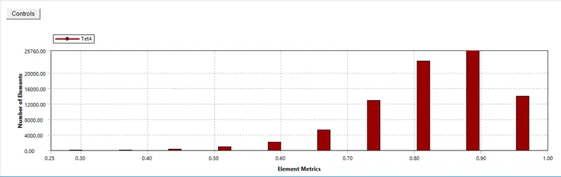
The minimum element quality is above 30 % & hence is acceptable.

C. SIMULATION SETUP

1. Solver: Steady

2. Type: Density-Based

3. Turbulence Model: SST k omega

4.Fluid: Air

5. Fluid Temperature: 300k

6. Boundaries:

• Inlet: Velocity = 50 m/s
• Outlet: Pressure = 0 Pa (Gauge Pressure)
• Lateral Faces & Top of Wind Tunnel: Symmetry
• Car Body & Bottom Face of Wind Tunnel:

Wall motion - Stationary Wall

Shear Condition - No-slip

7.Solution

• Method: Hybrid
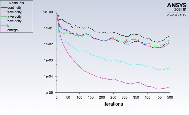
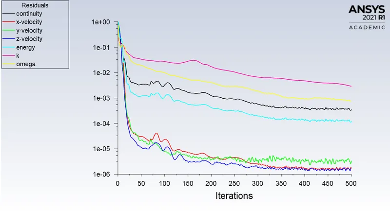
• Number Of Iteration: 500

8. Simulation Output

8.1. Residuals

D. POST-PROCESSING

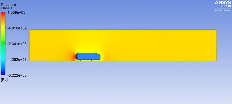
1. Pressure Contour

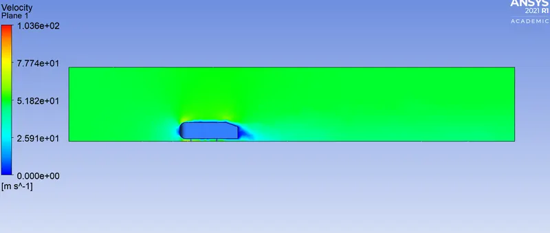
2. Velocity Contour

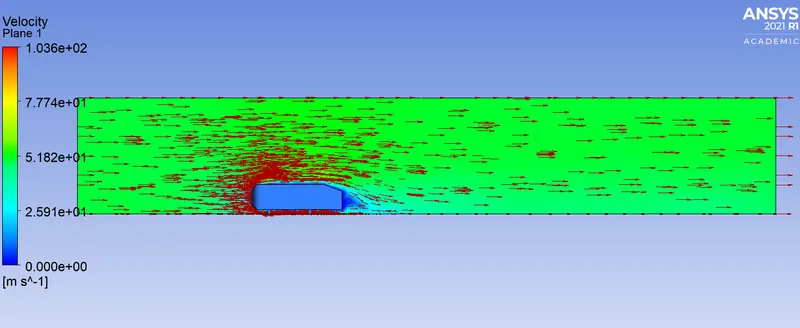
3. Velocity Vectors

4. Mesh Lines

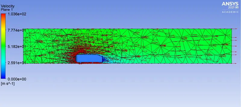
We can observe from the above contours that the obtained results are very coarse. Hence, we have to refine the mesh further.

Also, as the main objective of this setup is to analyze the flow parameters around the Ahmed Body, the refinement of the mesh should be mainly on the region surrounding it

Vll. REFINED MESH

As we know as the mesh is low it gives better results but simultaneously it also increases the computational time and computational memory. So for this case setup, we shall add another smaller encloser surrounding the Ahmed Body. So the second encloser will help us to further refine the region surrounding the Ahmed body.

SPACECLAIM GEOMETRY

1. Ahmed Body In Wind Tunnel

1.1 Model

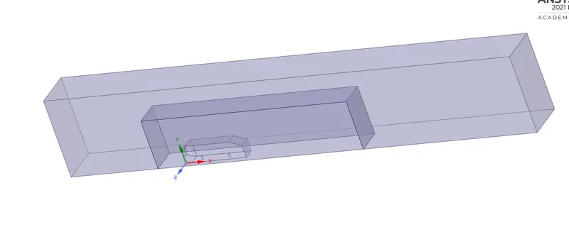
• Using the Split body command, the Ahmed body was split into 2 symmetrical halves for the main motive of reducing mesh count and saving the required time for computation
• An automatic interference check is conducted to avoid any mesh overlapping.
• The Ahmed body is suppressed for physics since the fluid will flow over it.
• Finally, the share topology option is activated to ensure fluid flow and data transfer over the 2 separated fluid domains.

CASE 1 - Y+ = 1 ----K-omega SST Model

First layer thickness = 0.00001432966 m

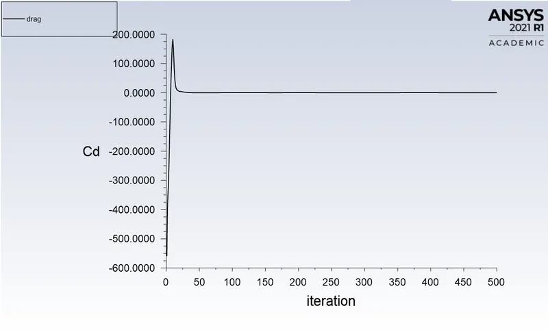
Drag Coefficient -- 0.38

MESHING

A. Refined Mesh

1. Named Selection

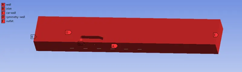
2. Enclosure 1

• Method: MultiZone
• Element Order: Linear
• Element Size : 0.1m

2. Encloser 2

• Body Sizing

Element Size = 0.05 m

• Edge Sizing

Element Size = 0.005 m

• Local Inflation Layer (Y plus=1 )

Number of Layers = 6

Growth Rate = 1.2

First Layer Thickness = 0.0000149607

3.Number of Nodes: 30279

4. Number of Elements: 104895

Figure 1 - Outer Enclosure

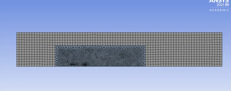
For the outer enclosure, the multizone method is selected. In this case, since the main computational domain is focused around the Ahmed Body, hence the refinement of the outer enclosure need not be too severe.

Hence, the multizone method which produces the highest quality mesh(i.e. hexahedral meshes)is the most appropriate mesh in the outer enclosure.

Figure 2 - Inner Enclosure

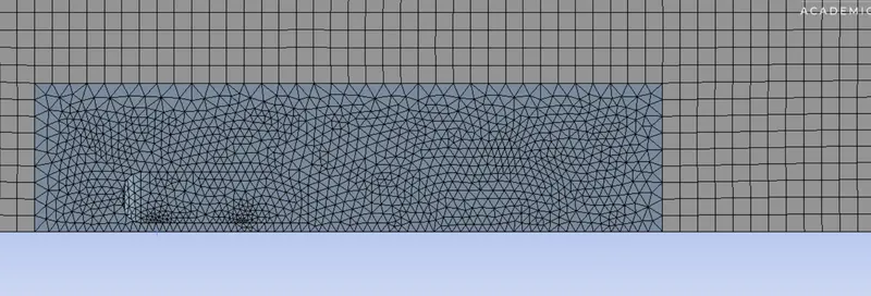
For the inner enclosure, the mesh size is reduced further. To analyze the flow parameters around the Ahmed Body, the mesh around the body can be refined further to increase the accuracy of the solution.

Figure 3 - Boundary Layered Mesh

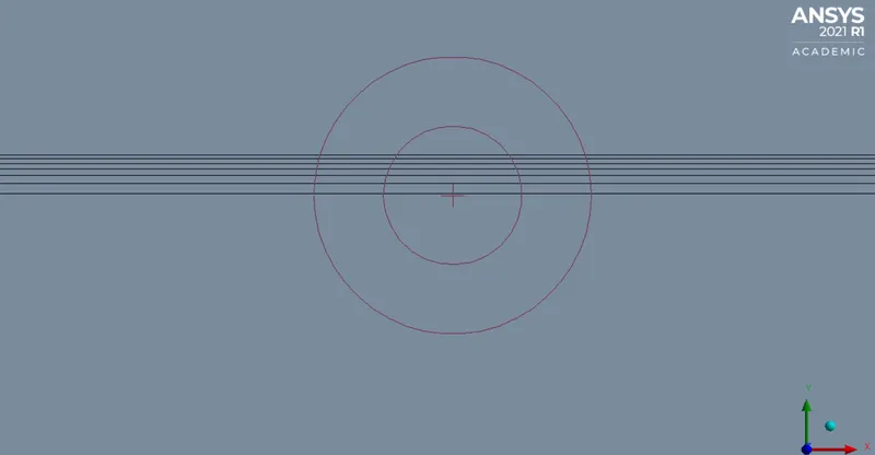
The final step is to add a boundary layer mesh to the Ahmed Body. The cells surrounding the boundary of the Ahmed Body have cell centers at different positions and are not ideal for simulating accurate solutions very close to the boundaries.

To avoid this, we have to add inflation layers to the boundaries of the Ahmed Body thus creating a boundary layered mesh that helps us to increase the accuracy of the solution.

Here we have used first layer thickness, which we calculated based on the Y plus(here 1) values, which is very small and need to zoom in to see it.

B. SIMULATION SETUP

The simulation setup is exactly that selected for the initial mesh. The only output of the simulation will change because of the change in the mesh size.

1.Reference Values

2. Residuals

3. Drag

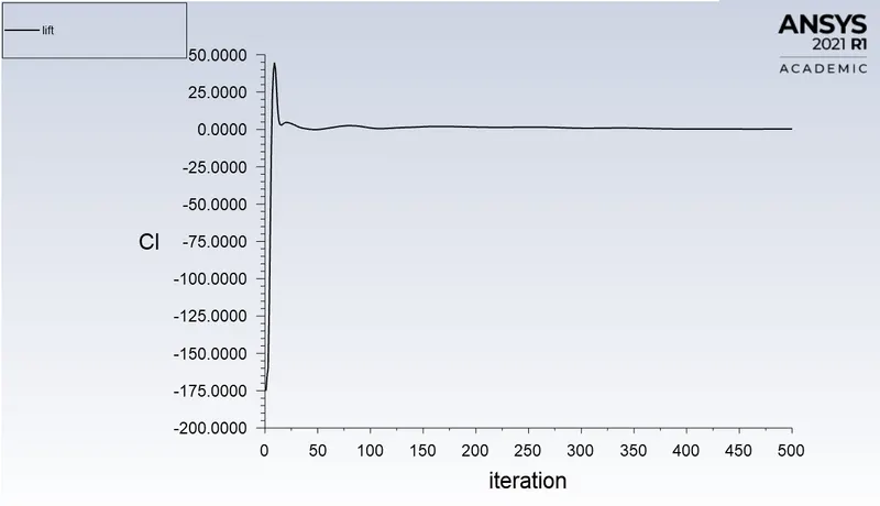
4. Lift

C. POST PROCESSING

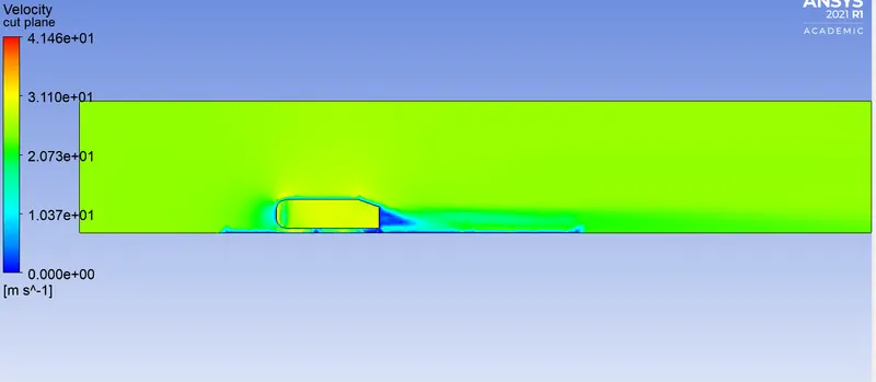
1.Velocity Contour

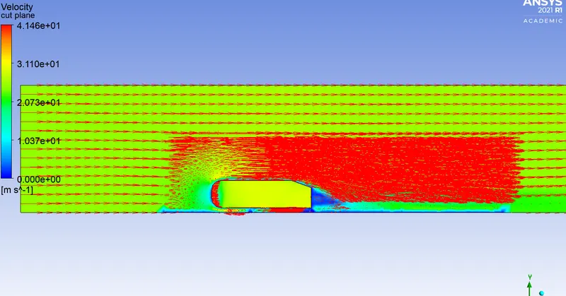
2. Velocity Vector

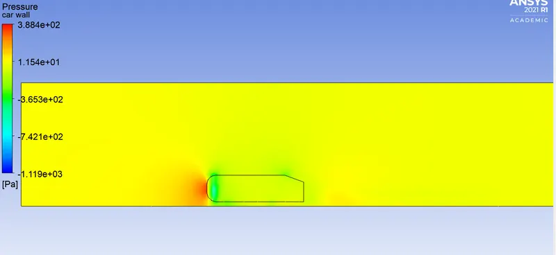
3. Pressure Contour

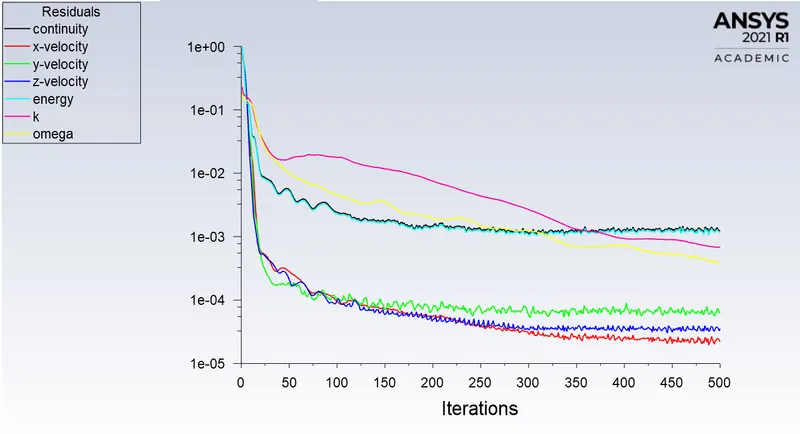
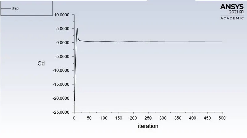
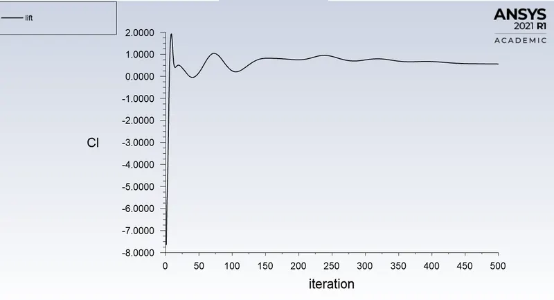
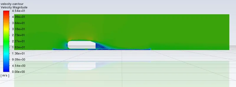
CASE 2 - Y+ = 5 ----K-omega SST Model

First layer thickness = 0.0000716483234694654 m

Drag Coefficient -- 0.32

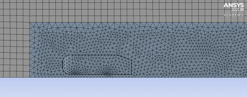
A. MESHING

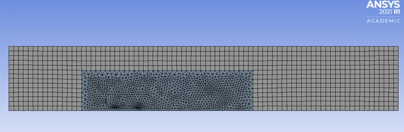
Number of Nodes: 30271

Numbers of Elements: 104751

B. SIMULATION SETUP

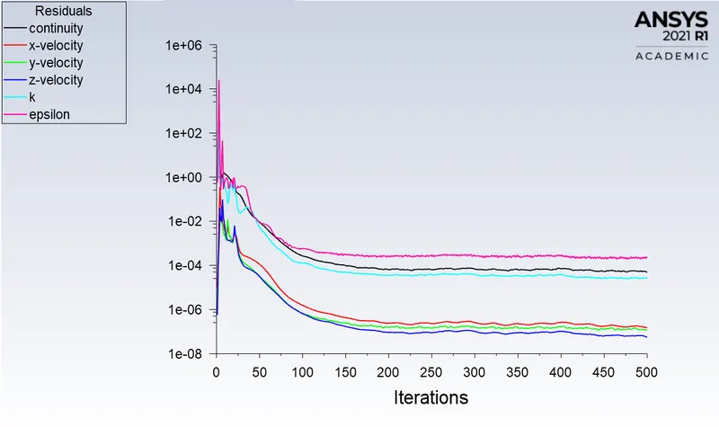
Simulation Output

1. Residuals

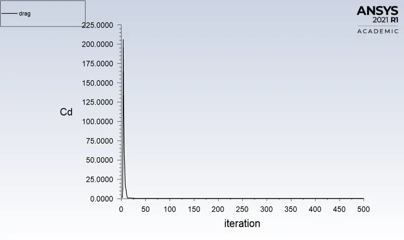
2. Drag

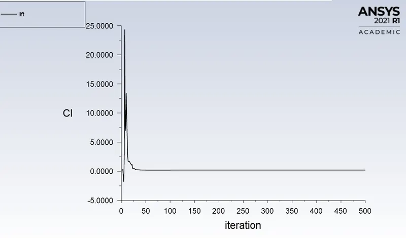
3. Lift

C. POST PROCESSING

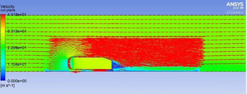
1. velocity Contour

2. Velocity Vector

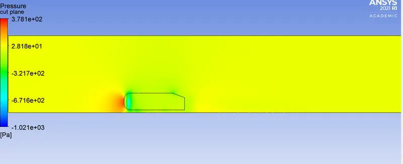
3. Pressure Contour

CASE 3 - Y+ = 30 ----K-epsilon Standard wall function

First layer thickness = 0.00042988994081679234 m

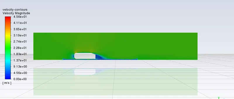
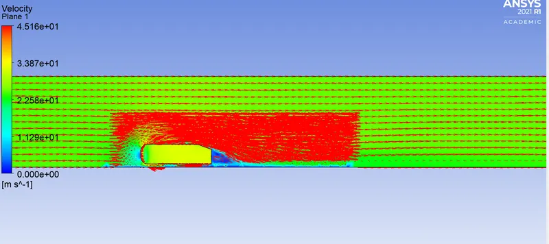
Drag Coefficient -- 0.36

A. MESHING

Number of Nodes: 30086

Number of Elements: 103828

B. SIMULATION SETUP

Simulation Output

1. Residuals

2. Drag

3. Lift

C. POST PROCESSING

1. Velocity contour

2. Velocity Vector

3. Pressure Contour

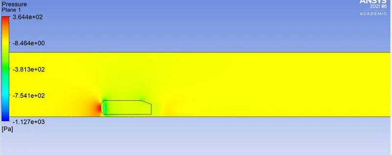
CASE 4 - Y+ = 100 ----K-epsilon Standard wall function

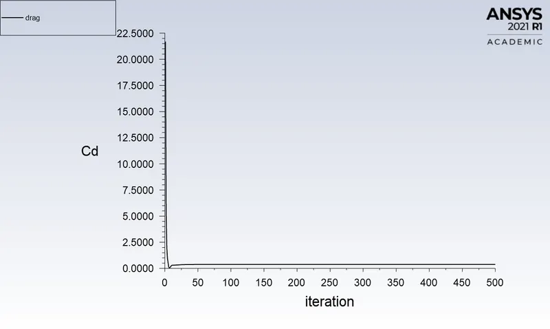
First layer thickness = 0.001432966469389308 m

Drag Coefficient -- 0.37

A. MESHING

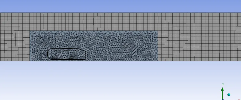
Number of Nodes: 29553

Number of Elements: 100915

B. SIMULATION SETUP

Simulation Outputs

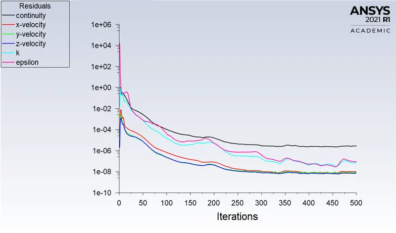
1. Residual

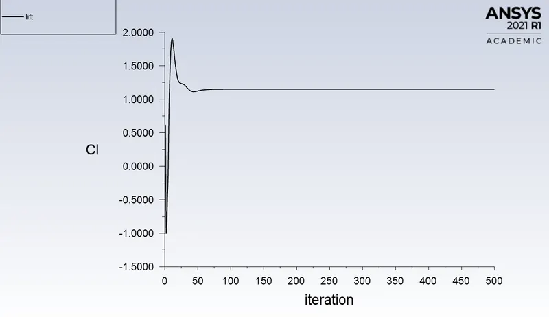
2. Drag

3. Lift

C. POST PROCESSING

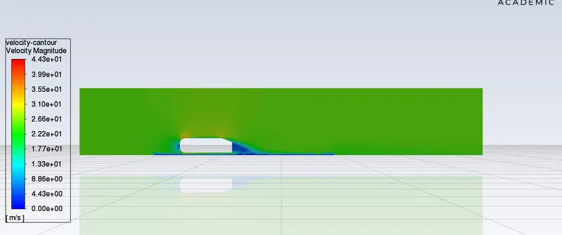
1. Velocity Contour

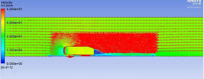
2. Velocity Vector

3. Pressure Contour

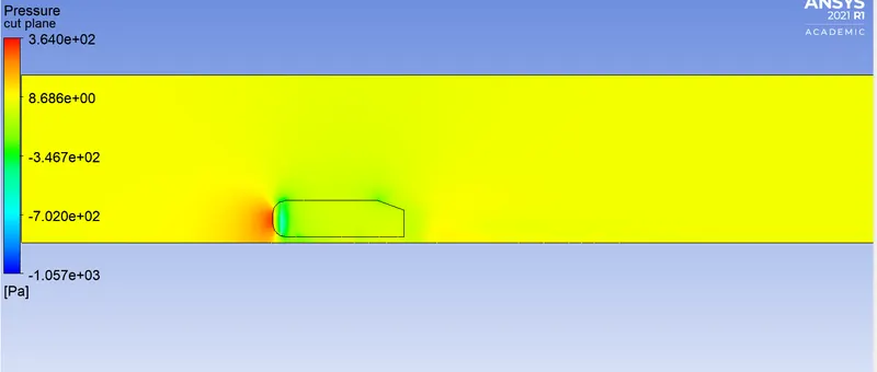
CONCLUSION: By observing the above simulation data and plot we can conclude that

1. The baseline mesh gives poor results.
2. As mesh size decreases the quality of mesh increases, as well as results, also become more precise and accurate.
3. With decreased mesh size, computational time increases.
4. The drag coefficient for Ahmed's body is 0.32 which is near to 0.33(theoretical) for fine mesh. Hence refined mesh gives a better result.
5. Changing Y+ values results in variable drag coefficient values.
6. Providing inflation layer capture flow better around the body.
7. The location of the flow separation point is very important as the flow starts recirculating from that point.
8. The negative pressure is created due to flow separation and recirculation of flow.