Finite Volume Method Literature Review

AIM: To describe the need for interpolation schemes and flux limiters in FVM.

THEORY: Discretization is the process of converting partial differential equations into Algebraic forms. The whole idea behind discretization is to get the solution at discrete points.

Methods of Discretization

1. Finite Difference Method
2. Finite Element Method
3. Finite Volume Method

FINITE VOLUME METHOD:

In the case of FVM, the problem domain is divided into several non-overlapping control volumes called Finite Volume. Finite volume is based upon the approximate solution of the integral form of the conservation equation. In form of an algebraic equation in the finite volume method, volume integrals in differential equations that contain a divergence term are converted into surface integral using the Gauss Divergence Theorem. These terms are then evaluated as flux at the surfaces of each finite volume. Because the flux entering a given volume is identical to that leaving the adjacent volume, these methods are conservative. Another advantage of the finite volume method is that it is easily formulated to allow for unstructured mesh. The method is used in many Computational Fluid Dynamics packages. 'Finite Volume ' refers to the small volume surrounding each node point on a mesh.

Features of FVM

1. FVM can accommodate any type of grid and hence it is naturally suitable for any type of grid.
2. Unstructured grid generation method and mesh partitioning techniques developed for Finite element Methods can be directly used in FVM.

TYPES OF FVM GRIDS

1. Cell Centered approach: Control volumes are defined by a suitable grid and computational nodes are assigned at the control volume center. It can be applied to both structured and unstructured grids. The cell-centered nodal value represents the mean over the control volume. This approach is the most commonly used in the Finite volume method.

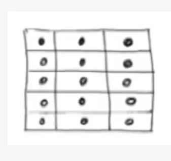Structured Grid.

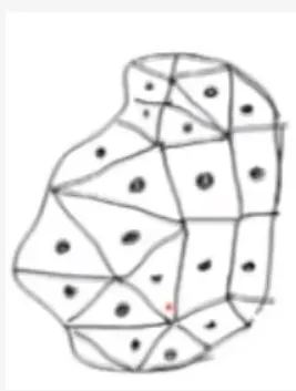Unstructured Grid.

2. Face-centered approach: Nodal locations are defined first and control volumes are then constructed around them so that the control volume's faces lie midway between the nodes. It can only be used with structured grids.

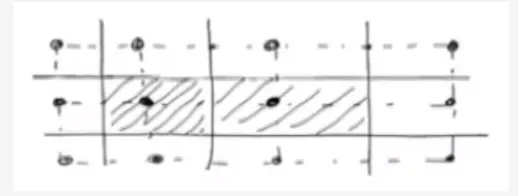
Approximation of Surface integral

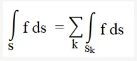
Net flux through the control volume boundaries is the sum of integral over the control volume faces, where 'it is the component of the convective or diffusive flux in the direction normal to the control volume.

INTERPOLATION METHODS

The approximation of surface and volume integrals requires values of the variable at a location other than the computational nodes of the control volume.

Values at these locations are obtained using the interpolation formula.

Various possibilities for interpolation are as follows.

1) Upwind interpolation

2) Linear interpolation

3) Quadratic upwind interpolation

4) Hybrid, TVD, and ENO interpolation schemes.

Flux Limiter

Flux limiters are used in high-resolution schemes i.e. numerical schemes used to solve the problem in science and engineering, particularly fluid dynamics, described by PDE. They are used in high-resolution schemes, such as the MUSCL scheme, to avoid the spurious oscillations(wiggles) that would otherwise occur with high order spatial discretization scheme due to shocks, discontinuities, or sharp changes in the solution domain. The use of flux limiters, together with an appropriate high-resolution scheme, makes the solution total variation diminishing (TVD).

Note that flux limiters are also referred to as slope limiters because they both have the same mathematical forms and both have the effect of limiting the solution gradient near shocks or discontinuities. In general, the term flux limiter is used when the limiter acts on system states(like pressure, velocity...etc).

Need for Interpolation schemes and Flux limiters in FVM

1. The Gauss divergence theorem simply states the outward flux of a vector field through a closed surface, is equal to the volume integral of the divergence over the region inside the surface.
2. This theorem is fundamental in the FVM, it is used to convert the volume integrals appearing in the governing equation into surface integrals.
3. The face values appearing in the convection and diffusive fluxes have to be computed by some form of interpolation from the centroid value of control volume at both sides of the face.
4. After spacial discretization, we can proceed with temporal discretization. By proceeding in this way we are using a method of lines(MOL).
5. The main advantage of the MOL method is that it allows us to select numerical approximations of different accuracy for spatial and temporal terms. Each term can be treated differently to yield different accuracies.