Week 7: Shock tube simulation project

SIMULATION OF SHOCK WAVES IN A SHOCK TUBE USING CONVERGE

l. OBJECTIVE

1. Simulate the propagation of shock waves through a shock tube.

2. Plot the pressure and temperature history in the entire domain.

3. Plot the cell as a function of time.

ll. INTRODUCTION

A shock tube is a device that is used to produce and confine shock waves. It consists of the high-pressure and low-pressure region which is separated by a diaphragm.

When the diaphragm is ruptured, compression waves are generated, propagating as a shock in the low-pressure region. At the same time, expansion or refraction waves are generated and travels back to the high-pressure region.

The stationary gases in the low-pressure area will experience a rise in pressure and temperature due to the formation of shock waves and they will start moving towards the walls of the tube. Since the shock wave travels at supersonic speed, it generates an expansion fan. An expansion fan consists of an infinite number of Manch waves that diverge from a sharp corner. Both the expansion fan ad the shock waves are reflected from the closed ends of the tube.

When the shock wave hits the closed end of the tube, it gets reflected. This reflected shock wave cancels the motion of gases in the low-pressure section initiated by the primary shock wave. The strength of the shock wave and expansion fan depends on the initial pressure ratio across the diaphragm and the physical properties f the gases present in the tube.

lll. SHOCK TUBE SIMULATION

A. Model

The dimensions of the tube = 0.2 x 0.01 x 0.01 m

The model considered in this project is as shown below -

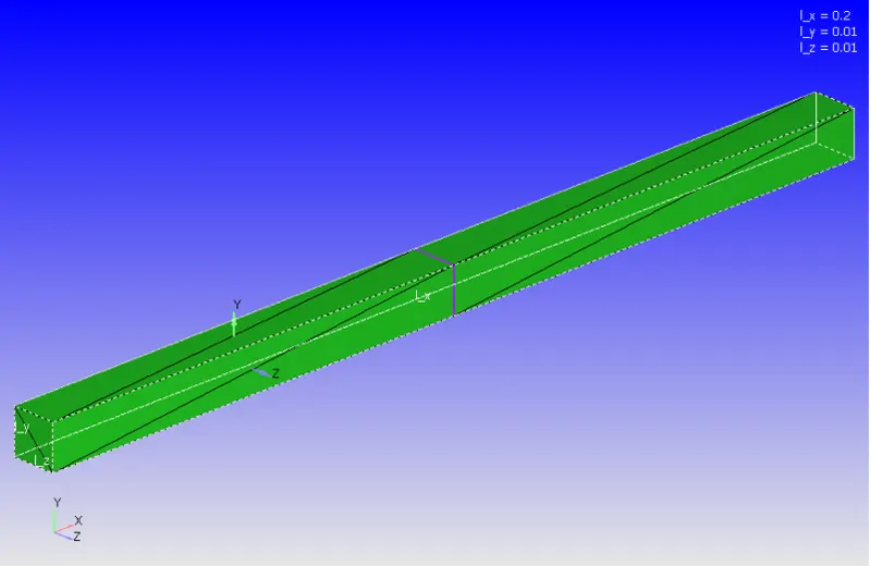
• Upon running a diagnosis check, it was noted that there were some non-manifold edge problems.
• This was due to the presence of a diaphragm inside the tube. This was deleted for this analysis. With the deletion, the problem of non-manifold edges disappeared.

B. Geometry Setup And Boundary Flagging

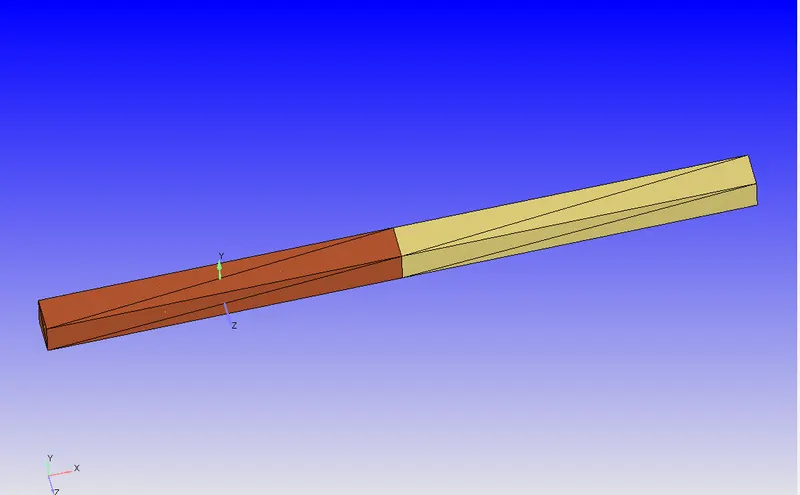
The geometry is set up and the boundaries are flagged in converge studio as shown in the figure below-

C. CASE SETUP

1. Application Type: Time Based

2. Materials:

• Predefined Mixture: Air
• Gas Simulation: Default
• Species:
  • Gas: `O_2` and `N_2`

3. Solver: Transient

4. Simulation Time Parameters:

• Start Time: 0 s
• End Time: 0.025 s
• Initial time-step: 1e-9 s
• Minimum time-step: 1e-9 s
• Maximum time-step: 1 s

5. Region and Initialization:

• High-Pressure Region:
  • Stream ID: 0
  • Temperature: 300 K
  • Pressure: 600000 Pa
  • Species: Nitrogen
    • Mass fraction of Nitrogen: 1
• Low-Pressure Region:
  • Stream ID: 0
  • Temperature: 300 K
  • Pressure: 101325 Pa
  • Species: Oxygen
    • Mass fraction of Oxygen: 1

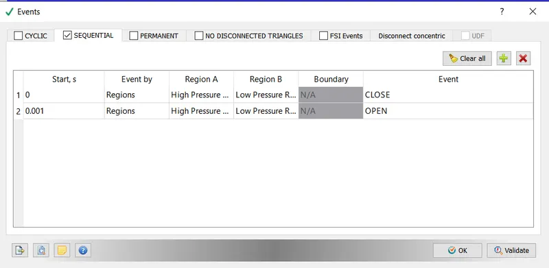
6. Events

7. boundary Conditions:

Boundary	Region	Boundary Type	Dirichlet Boundary Condition
High Pressure	High-Pressure Region	Wall	Velocity: Stationary and Slip Temperature: 300 K
Low Pressure	Low-Pressure Region	Wall	Velocity: Stationary and Slip Temperature: 300 K

8. Physical Models:

• Turbulence Model: RNG `k epsi`

9. Grid Control:

• Base Grid:
  • dx = dy = dz = 0.001 m
• Adaptive Mesh Refinement: AMR Group 1
  • Active Region:
    • High-Pressure Region
    • Low-Pressure Region
  • Species: `N_2`
    
    • Maximum Embedding Level: 3
    • Timing Type: Permanent
    • Sub-Grid Scale Criteria: 0.001

10. Output Files:

• Time interval for writing 3-D output: 1e-5 s
• Time interval for writing text output: 1e-6 s
• Time interval for writing restarting output: 0.0005 s

E. OUTPUTS, RESULTS, AND INFERENCE

1.Mesh

Converge monitors the curvature of the fluid property in the AMR and refines the mesh when the property curvature variation between the consecutive grid is more than the defined SGS value. This is done to capture the flow properties in the shock flow region accurately.

Animation 1 - Mesh Generation with Adaptive Mesh Refinement

2. Flow properties Contour Animation

Animation 2.1 - Mass Fraction of Nitrogen And Temperature Contour

When the diaphragm ruptures, the shock wave pushes the nitrogen gas towards the low-pressure region and compresses the oxygen gas. But before the gases could reach the other end of the tube, the reflected shock wave pushes the nitrogen gas in the opposite direction thereby changing the flow direction. That wave is again reflected from the other end of the tube and the process repeats until the intensity of the shock wave decreases and attains a steady state.

The temperature contour shows that due to the shock wave, there is a sudden increase in the temperature at the end of the shock tube i.e. in the high-pressure region. Similarly, the temperature reaches a minimum at the other end of the shock tube i.e. in the low-pressure region.

Animation 2.2 - Pressure And Velocity Contour

The pressure contours show that as the shock wave travels to any end of the tube, the pressure keeps decreasing until the wave gets reflected which is followed by a sudden increase in the pressure and the process continues until the intensity of the shock waves decreases and attains a steady-state.

The velocity contour directly depicts the speed of the shock wave, which changes its direction at zero velocity and then increases as it moves from one end to the other end. Also, note that the shock wave has a high initial velocity which keeps decreasing as the intensity of the shock waves reduces.

3. Plots

Figure 3.1 - pressure Profile

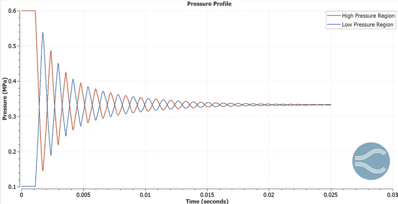
The pressure is initially 6 bar in the high-pressure region and 1 atm in the low-pressure region. Due to the sudden rupturing of the diaphragm and the presence of a high-pressure difference between the two regions, shock waves are created and propagated in the shock tube.

As the shock wave propagates the pressure keeps on decreasing cyclically, due to the damping effects, until a steady state is achieved. It can be seen that at the end of the 25 ms, the pressure attains a steady state of approximately 3.33 bar.

Figure 3.2 - Temperature Profile

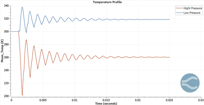
Initially, the temperature throughout the shock tube is 300 K. AFter the shock waves are generated, the temperature in both regions starts varying cyclically. The temperature in the low-pressure region varies between 300 K and the global maximum (in this case 340 K) and the temperature in the high-pressure region varies between 300 K and the global minimum ( in this case 200 K) before attaining a steady state of approximately 287 K.

Figure 3.3 - Total Cell Count Variation

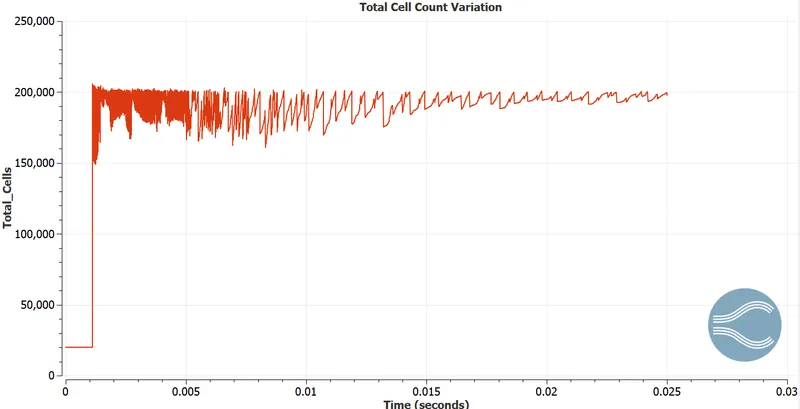
The total cell count is initially constant at 20,000. After the diaphragm is ruptured, the cell count increases to properly compute the changes in species concentration in the shock wave region through adaptive mesh refinement. the total cell count varies continuously throughout the time interval until the simulation attains a steady-state, where the variations are observed much more slowly.

lV. CONCLUSION

The behavior of shock waves in a shock tube due to the rupturing of a diaphragm has been successfully simulated and analyzed. Results from shock tube experiments can be used in a variety of applications such as to develop and validate a numerical model of the response of a material or object to an ambient blast wave without shrapnel or flying debris.

Shock tubes can be further developed into shock tunnels, with an added nozzle and dump tank. The resultant high-temperature hypersonic flow can be used to simulate atmospheric re-entry of spacecraft or hypersonic craft.