SIMULATING FLOW THORUGH A MIXING TEE
AIM: To simulate the flow of air through a mixing tee and study the mixing effectiveness of this in pipes of different lengths and different momentum ratios.
Theory: In industrial process engineering, mixing is a unit operation that involves the manipulation of a heterogeneous physical system with the intent to make it more homogeneous. Mixing is performed to allow heat or mass transfer to occur between one or more streams, components, or phases. Modern industrial processing almost always involves some form of mixing. Mixing Tess is a type of mixing mechanism. Mixing Tee utilizes a specifically engineered internal geometry to efficiently mix two fluid streams into one combined stream. Mixing tees are widely used in the petrochemical, HVAC industry, etc, in which two fluids streams with different physical or chemical properties mix together.
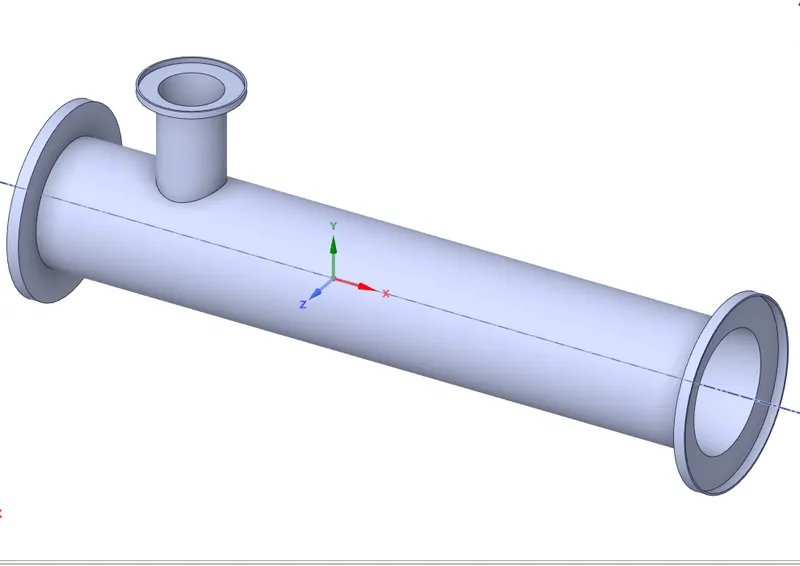
Hot air flowing in the main pipe is mixed with cold air flowing through a tee. The standard deviation of temperature is computed to quantify the degree of mixing. The velocity and temperature fields are also computed. The effects of the mesh size, turbulence model on results were examined. For this, we have created two versions of the mixing tee. One of them is longer than the other.
For this, we have created two versions of the mixing tee. One of them is longer than the other.
It is set up as steady-state simulations to compare the mixing effectiveness when hot inlet temperature is `36^0 C` & the cold inlet is at `19^0C`.
1. Case 1
Short mixing tee with a hot inlet velocity of 3m/s.
Momentum ratio of 2,4.
2. Case 2
Long mixing tee with a hot inlet velocity of 3m/s.
Momentum ratio of 2,4.
The momentum ratio is defined as the ratio of velocity at the cold inlet to the velocity at the hot inlet.
CASE setup-
CAD cleanup/Pre-processing-SpaceClaim.
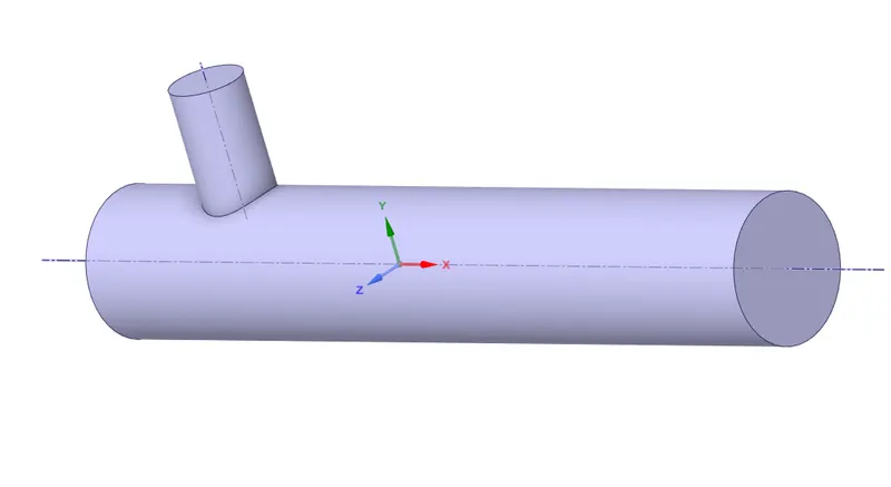
The CAD model is imported into the SpaceClaim to extract the flow volume field from the model. The extracted volume is shown below:
Mesh
The boundary names are applied in this section and a mesh is generated.
Setup
In this section, we apply different boundary conditions like inlet, outlet boundary conditions. Turbulence models are set up like K-epsilon or K- omega for solving the turbulent mixing of air. The number of iterations is set in this section.
CFD-Post
Post-processing is carried in this section in which different contours are set up to visualize the properties (such as Temperature, Velocity, etc.) for which simulation is run.
CASE 1 - SHORT TEE
a) For inlet velocity of 3m/s and momentum ratio of 2
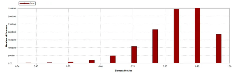
A mesh element metric that identifies the quality of the mesh is employed and it can be seen that the elements of the lowest quality employed are minimal. Most of the elements have quality in the range of 0.7 to 1. Hence the mesh is of acceptable quality.
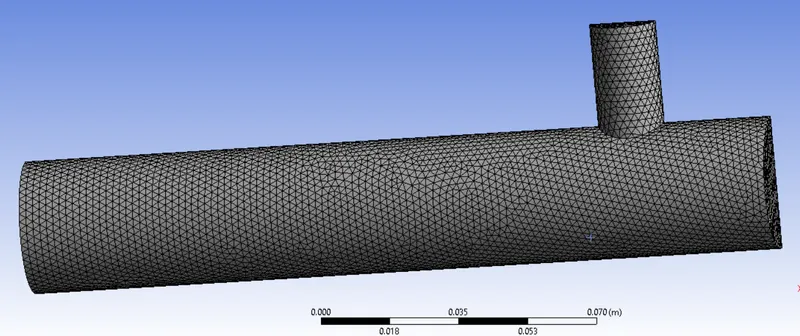
MESH of size = 0.002m
Grid Independence Study:
We need to ensure the results we obtain are independent of mesh size to achieve more confidence in our results and also reduce the computational time. A coarse mesh, finer mesh, and very fine mesh were generated and compared with the results which are tabulated below.
| Mesh Type | No of Elements | Element Size |
| Coarse | 12745 | 7mm |
| Fine | 14228 | 5mm |
| Very Fine | 105618 | 2mm |
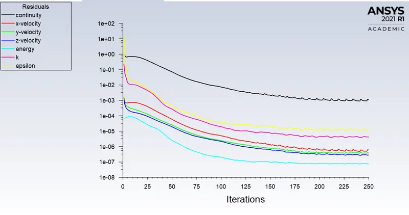
Residual Plot:
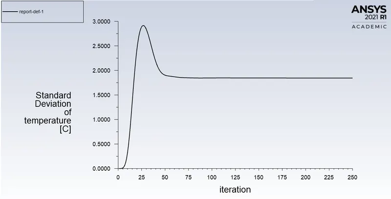
Standard-Deviation of Temperature Plot:
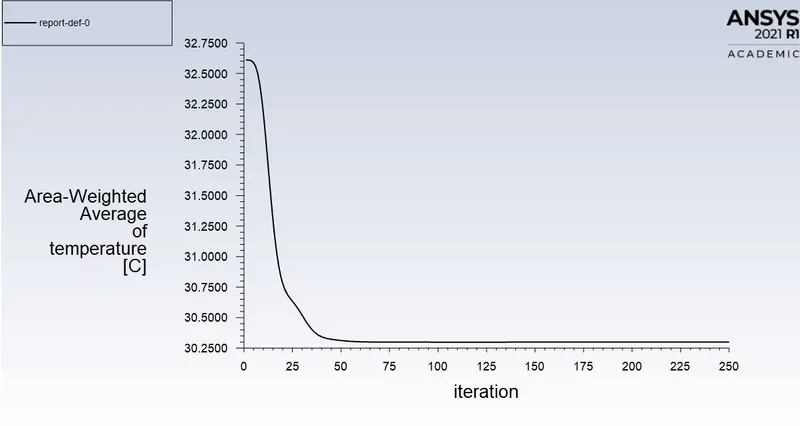
AWA of Temperature Plot:
Contours-
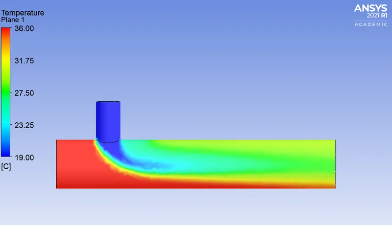
1) Temperature:
2) Velocity:
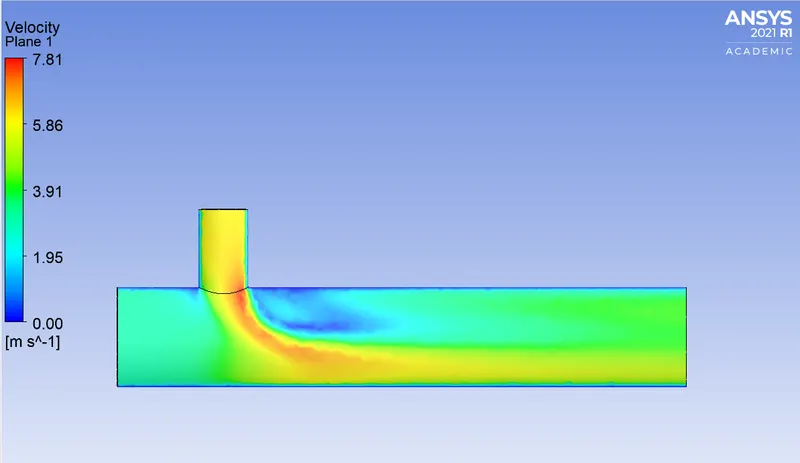
b)For inlet velocity of 3m/s and momentum ratio of 4
Residual plot:
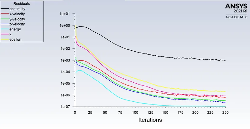
Standard-Deviation of Temperature Plot:
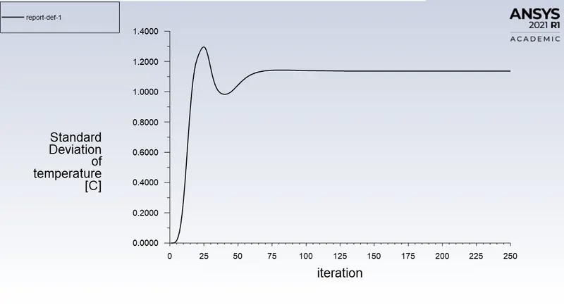
AWA of Temperature Plot:
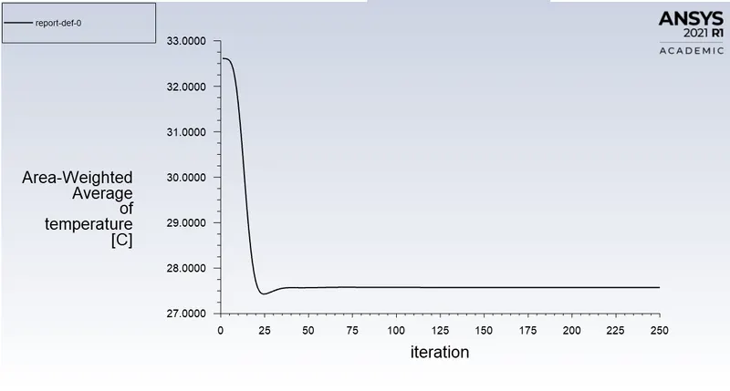
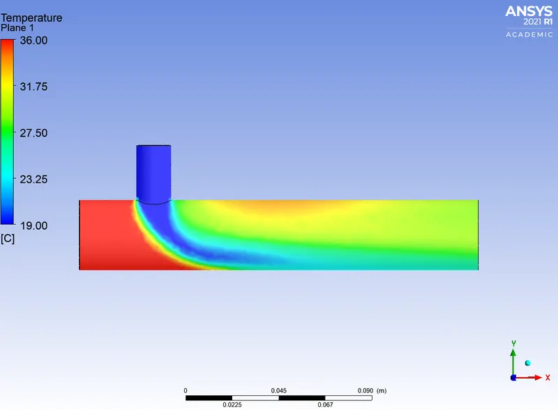
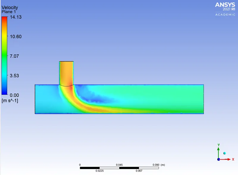
Contours:
1) Temperature:
2) Velocity:
CASE 2 - LONG TEE
a) For inlet velocity of 3m/s and momentum ratio of 2
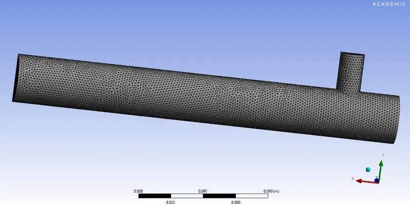
A mesh element metric that identifies the quality of the mesh is employed and it can be seen that the elements of the lowest quality employed are minimal. Most of the elements have quality in the range of 0.7 to 1. Hence the mesh is of acceptable quality.
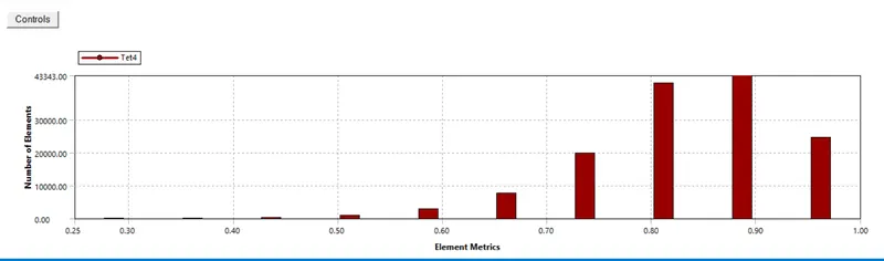
MESH of size = 0.002m
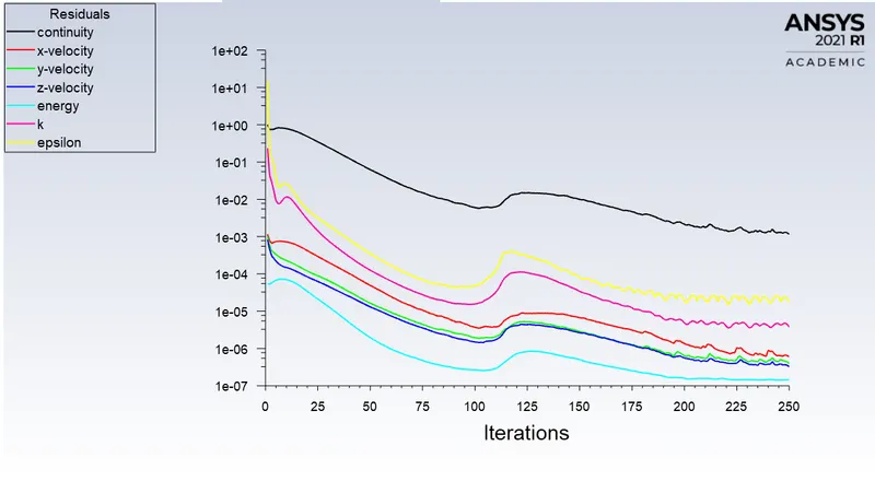
Residual:
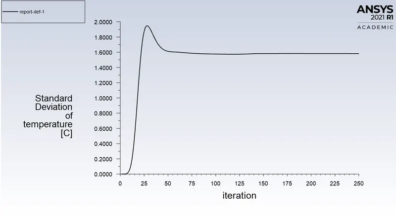
Standard Deviation:
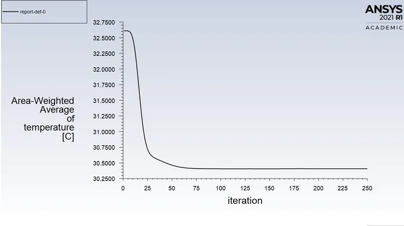
AWA of Temperature:
Contour-
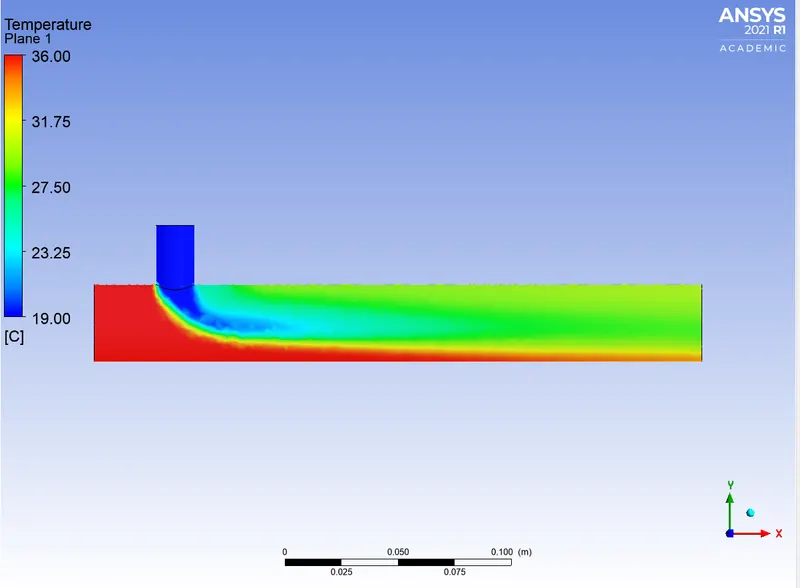
1) Temperature:
2) Velocity:
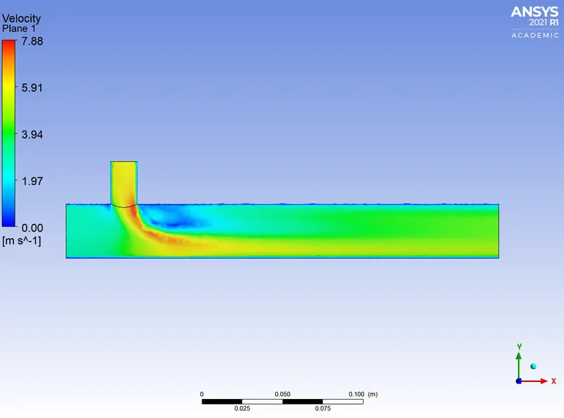
b) For inlet velocity of 3m/s and momentum ratio of 4
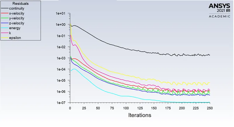
Residual:
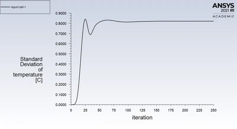
Standard Deviation:
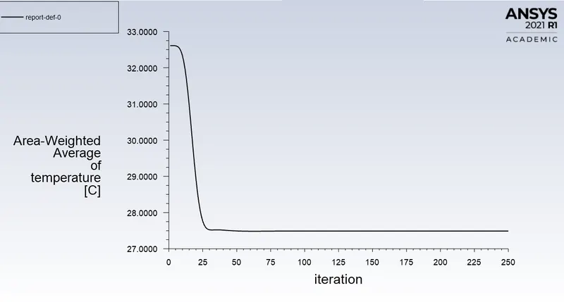
AWA of Temperature:
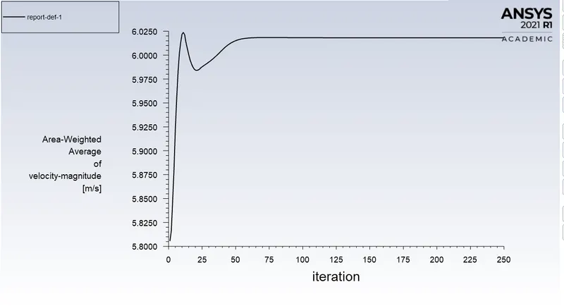
AWA of Velocity:
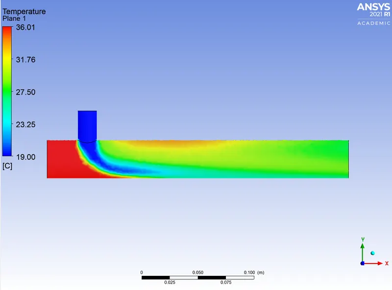
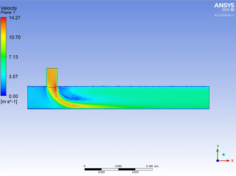
Contour:
1) Temperature:
2) Velocity:
Comparison of all cases:
| Case | Cell Count | AWA of Temperature(c) | Number of Iteration |
| Short Tee- Momentum Ratio 2 | 105618 | 30.29 | 250 |
| Short Tee- Momentum Ratio 4 | 105618 | 27.57 | 250 |
| Long Tee- Momentum Ratio 2 | 140025 | 30.40 | 250 |
| Long Tee- Momentum Ratio 4 | 140025 | 27.48 | 250 |
CONCLUSION:
1. As seen in Case 1-A and Case 1-B, the temperature at the outlet drops down significantly due to the high velocity of cold air from the inlet. This is possible due to turbulent mixing at the tee joint between hot air and cold air because of the high velocity of cold air, which is not possible in the case of low-velocity cold air.
2.The temperature contour at the outlet for short tee cases shows that some of the high-temperature flow sips through without properly mixing with the flow. Whereas, in the temperature contour of long tee cases, the high temperatures flow thoroughly mixes with the rest of the flow.
3. Therefore, we can recommend using the long tee and high-velocity inlet for application. This is because we have a low standard derivation in the case of long tee compared to the short tee for both momentum ratios.
4. K-epsilon model predicts well far from boundaries (wall) and K- omega model predicts well near the wall. Even though it depends on Y+. Therefore, the K-epsilon model is majority used for free flow away from the wall and as in this project, there is no dealing with the wall of the mixing tee for change in temperature along the length of it, so the K-epsilon model was chosen for further simulations.