Week 8: Literature review - RANS derivation and analysis

LITERATURE REVIEW - REYNOLDS AVERAGED NAVIER-STROKE (RANS) EQUATIONS DERIVATION AND ANALYSIS.

l. OBJECTIVE

1. Understanding the challenges of simulating turbulent flow and the need for turbulence models.

2. Derivation of RANS equations by the application of Reynolds decomposition on the time-averaged Navier-Stroke equation.

3. Understanding the stresses which define the transfer of momentum from the boundary layer and the parameters associated with it.

ll. INTRODUCTION

1. Turbulent Flow

Turbulent flow is a type of fluid flow in which the fluid undergoes irregular fluctuations, or mixing, in contrast to laminar flow, in which the fluid moves in smooth paths or layers.. in turbulent flow, the speed of the fluid at a point is continuously changing in both magnitude and direction. The flow of wind and rivers is generally turbulent in this sense, even if the currents are gentle. The air or water swirls and eddies while its overall bulk moves along a specific direction.

There are several challenges that we need to overcome to model an accurate turbulent flow-

1. Unsteady aperiodic motion.
2. Fluid properties exhibit random spatial variations.
3. Strong dependence on initial conditions.
4. Contains a wide range of scales(eddies).

2. Navier-Stokes Equation

The Navier-Stokes equations describe the motion of fluids, through the conservation of mass, momentum, and energy.

The equations are non-linear, which creates a continuous spectrum of different flow features. this spectrum contains very large integral scales and very small dissipation scales. The simultaneous representation of both large and small scales makes for a very large computational problem.

Current computational resources limit the number of small features that can be accurately simulated. Therefore, there is a need to approximate the Navier-Stokes equations on a computational grid using discrete physical points or basic functions.

Figure - Methods to simulate Turbulent Flow

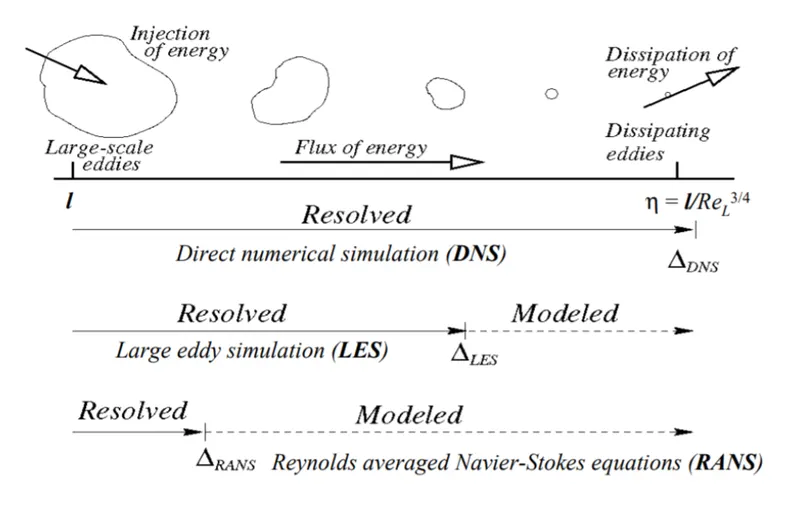
Three basic methodologies are prevalent in turbulence application and research:

2.1. Reynolds Averaged Navier-Stokes (RANS)

1. Solvers equations for an ensemble-averaged velocity field and the magnitude of turbulent fluctuations.
2. RANS modeling has a low computational cost and can be used for highly complex flow geometries.
3. When combined with empirical information, it can be highly used for engineering applications and to parameterize near-wall behaviors.
4. Only steady flow phenomena can be explored with the full advantage of computational reductions.
5. Models are not universal since the dynamic consequences of all scales must be represented.
6. Most accurate turbulence models give rise to highly complex equations sets, which can lead to numerical formulation and convergence issues.

2.2. Large Eddy Simulations(LES)

1. Navier-Stokes equations are numerically solved without any turbulence model. This means that the whole range of spatial and temporal scales of the turbulence must be resolved.
2. Very high memory and computational time costs.
3. Accuracy is only limited by computational capabilities since errors are ger=nerally only due to sensitivity to perturbations or accumulated round-off errors.
4. All aspects of the flow in time and space are available, which is not possible for experiments (i.e, 3-D velocity and scalar fields).
5. Restricted to low-Re flows with relatively simple geometries.

3. Reynolds Decomposition

Reynolds decomposition is a mathematical technique used to separate the mean value of quantity from its fluctuations.

`u_i(x,y,z,t)_text(instantaneous) = baru_i(x,y,z,t)_text(fluctuating)`

Figure - Graphical Representation of Velocity Average and Fluctuating Components

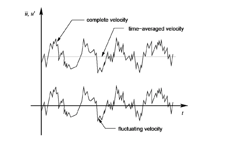
Reynolds decomposition allows the simplification of the Navier-Stokes equations by substituting in the sum of steady component and perturbations to the velocity profile and taking the mean value. The resulting equation contains a non-linear term known as the Reynolds stress which gives rise to turbulence.

lll. DERIVATION OF REYNOLDS AVERAGED NAVIER-STOKES (RANS) EQUATIONS

1. Simplified Navier-Stokes Equations Inside A Boundary Layer

The RANS equations are required to describe the behavior of turbulent flows. They are derived by time-averaging the Navier-Stokes equations.

The Navier-Stokes equations inside a boundary layer can be represented as follows -

1.1. Continuity Equation:

`(delu)/(delx)+(delv)/(dely)=0`

1.2. Momentum Equation:

`rho[(delu)/(delt)+u(delu)/(delx)+ v(delu)/(dely)]=-(delp)/(delx)+mu(del^2u)/(dely^2)`

1.3. Energy Equations

`rhoc[(delT)/(delt)+u(delT)/(delx)+v(delT)/(dely)]=k(del^2T)/(delx^2)+mu((delu)/(dely))^2`

2. Reynolds Decomposition On The System Variables.

Let `u` and `v` represent the instantaneous velocity of the fluid in the x and y directions respectively. Also `p` represents the pressure acting on the fluid at any instant.

According to the concept of Reynolds decomposition, the dependent variables of the system are decomposed into their corresponding mean and fluctuating parts-

`u = baru + u',v=barv+v'` and `p=barp+p'`

Analogously, this can be applied for the density and the temperature. However, the density and temperature are assumed to be constant in this derivation.

3. Assumptions In The Derivation Of RANS Equations

Assumption 1:

The chosen averaging method takes the mean values at a fixed place in space and is averaged over a time span that is large enough for the mean values to be independent of it.

`baru= 1/(Deltat)int_(t_o)^((t_0)+ Deltat) udt`

Assumption 2:

The time-averaged values of the fluctuating values are defined as zero.

`bar(u')= 1/(Deltat)int_(t_o)^(t_0+ Deltat) u'dt=0`

Assumption 3:

Boundary Layers are very thin compared to the size of the plate. Hence, the gradients of the velocity component along the x-direction are very small compared to those in the y-direction.

Hence, `1/(Deltat)int_(t_o)^((t_0)+ Deltat) (del(u')^2)/(delx)dt=0`

4. Reynolds Decomposition on the Continuity Equations

`(delu)/(delx)+(delv)/(dy)=0`

Applying Reynolds decompostion

`(del(baru+u'))/(delx)+(del(barv+v'))/(dely)=0`

Time-averaging the above equations

`1/(Deltat)int_(t_0)^(t_0+Deltat)[(del(baru+u'))/(delx)+(del(barv+v'))/(dely)]dt=0`

`1/(Deltat)int_(t_0)^((t_0)+Deltat)(delbaru)/(delx)dt+1/(Deltat)cancel(int_(t_0)^((t_0)+Deltat)(delu')/(delx)dt)+1/(Deltat)int_(t_0)^((t_0)+Deltat)(delbarv)/(dely)dt+1/(Deltat)cancel(int_(t_0)^((t_0)+Deltat)(delv')/(dely)dt)=0`

`1/(Deltat)(delu)/(delx)int_(t_0)^(t_0+Deltat)dt+ 1/(Deltat)(delbarv)/(dely)int_(t_o)^(t_0+Deltat)dt=0`

`1/(Deltat)(delbaru)/(delx)[(t_0+Deltat)-t_0]+1/(Deltat)(delbarv)/(dely)[(t_0+Deltat)-t_o]=0`

`(delbaru)/(delx)+(delbarv)/(dely)=0-----}Equation 1`

Hence, we get the continuity equations in terms of the time-averaged quantities.

5. Reynolds Decomposition on the Momentum equation

`rho[(delu)/(delt)+u(delu)/(dx)+v(du)/(dely)]= - (delp)/(delx)+mu(del^2u)/(dely^2)`

`(delu)/(delt)+u(delu)/(dx)+v(du)/(dely)=-1/rho(delp)/(delx)+mu/rho(del^2u)/(dely^2)`

`(delu)/(delt)+u(delu)/(dx)+v(du)/(dely)=-1/rho(delp)/(delx)+v(del^2u)/(dely^2){text(since Kinematic Viscosity,) v=mu/rho}`

Adding `mu[(delu)/(delx)+(delv)/(dely)]` to both sides

`(delu)/(delt)+u(delu)/(dx)+v(du)/(dely)+mu[(delu)/(delx)+(delv)/(dely)]=-1/rho(delp)/(delx)+v(del^2u)/(dely^2)+u[ubrace(cancel[(delu)/(delx)+(delv)/(dely)])_("(From Continuity Equations")]`

`(delu)/(delt)+2u(delu)/(delx)+v(delu)/(dely)+u(delv)/(dely)=-1/rho(delp)/(delx)+v(del^2u)/(dely^2)+0`

`(delu)/(delt)+(delu^2)/(delx)+(deluv)/(dely)= -1/rho(delp)/(delx)+v(del^2u)/(dely^2)`

`{text(since)(del(uv))/(dely)=u(delv)/(dely)+v(delu)/(dely)text(and)(delu^2)/(delx)=2u(delu)/(delx)}`

Time-averaging the above equation and performingReynolds decompostion-

`1/(Deltat)int_(t_o)^(t_0+Deltat)[(del(baru+u'))/(delt)+(del(baru+u')^2)/(delx)+(del(baru+u')(barv+v'))/(dely)]dt=1/(Deltat)int_(t_0)^(t_0+Deltat)``[-1/rho(del(barp+p'))/(delx)+v(del^2(baru+u'))/(dely^2)]dt`

`1/(Deltat)int_(t_0)^(t_0+Deltat)(delbaru)/(delt)dt+1/(Deltat)cancel(int_(t_0)^(t_0+Deltat)(delu')/(delt)dt)+1/(Deltat)int_(t_0)^(t_0+Deltat)(del(baru)^2)/(delx)dt+1/(Deltat)cancel(int_(t_0)^(t_0+Deltat)(del(2baru)(u'))/(delx))dt+1/(Deltat)int_(t_0)^(t_0+Deltat)(del)/(delx)+``1/(Deltat)int_(t_0)^(t_0+Deltat)(del(barubarv))/(dely)dt+1/(Deltat)cancel(int_(t_0)^(t_0+Deltat)(del(baruv'))/(dely)dt)+1/(Deltat)cancel(int_(t_0)^(t_0+Deltat)(del(u'barv))/(dely)dt)+1/(Deltat)int_(t_0)^(t_0+Deltat)(del(u'v'))/(dely)dt`

`=1/(Deltat)int_(t_0)^(t_0+Deltat)-1/(rho)(del(barp))/(delx)dt+1/(Deltat)cancel(int_(t_0)^(t_0+Deltat)-1/(rho)(del(p'))/(delx)dt)+int_(t_0)^(t_0+Deltat)v(del^2baru)/(dely^2)dt+1/(Deltat)cancel(int_(t_0)^(t_0+Deltat)v(del^2u')/(dely^2)dt)`

`(delbaru)/(dt)+(del(baru)^2)/(delx)+(del(barubarv))/(dely)+1/(Deltat)int_(t_0)^(t_0+Deltat)(del(u')^2)/(delx)dt+1/(Deltat)int_(t_0)^(t_0+Deltat)(del(u'v'))/(delx)dt= -1/(rho)(delbarp)/(delx)+v(del^2baru)/(dely^2)`

`(delbaru)/(delt)+(del(baru)^2)/(delx)+(del(barubarv))/(dely)=-1/rho(delbarp)/(delx)+v(del^2baru)/(dely^2)-ubrace(1/(Deltat)cancel(int_(t_0)^(t_0+Deltat)(del(u')^2)/(delx)dt))_("From Assumption3")-1/(Deltat)int_(t_0)^(t_0+Deltat)(del(u'v'))/(dely)dt`

Therefore,

`(delbaru)/(delt)+(del(baru)^2)/(delx)+(del(barubarv))/(dely)=-1/(rho)(delbarp)/(delx)+v(del^2(baru))/(dely^2)-1/(Deltat)int_(t_0)^(t_0+Deltat)(del(u'v'))/(dely)dt`

Rearranging and simplifying-

`(delbaru)/(delt)+(del(baru)^2)/(delx)+(del(barubarv))/(dely)=-1/(rho)(delbarp)/(delx)+1/(rho)(del)/(dely)[mu(delbaru)/(dely)-(rho)/(Deltat)int_(t_0)^(t_0+Deltat)(u'v')dt]`

`ubrace((delbaru)/(delt)+(del(baru)^2)/(delx)+(del(barubarv))/(dely))_("Inertial Terms")=ubrace(-1/rho(delbarp)/(delx))_("Pressure Term")+ubrace(1/rho(del)/(dely)[ubrace(mu(delbaru)/(dely))_("Shear Stress")-ubrace(rhobar(u'v'))_("Reynolds Stress")])_("Momentum Diffusion Terms")---}text(Equation 2)`

lV. INFERENCES

We can observe that when we apply Reynolds decomposition on the momentum equation, the derived RANS equation has an additional term that represents the effect of the turbulent fluctuations on the given velocity and pressure fields. This term is the Reynolds stress and can be expressed as follows-

`tau_text(turbulence)= -bar(rhomu'v')`

Note that the viscous shear stress is caused by the velocity of the fluid as a result of intermolecular forces and hence is a property of the fluid, whereas Reynolds stress results from the turbulent transport of the momentum. The momentum flux in Reynolds stress causes deformation of a fluid parcel and is not because of the existence of a real tangential force as in viscous stress. Hence, Reynolds stress is a property of flow and is dependent on the flow variables.

The derived RANS equations lead to the closure problem in turbulence theory. The closure problem occurs when there are more unknowns than there are equations, ans this leads to the need for modeling to produce a closed system of equations.

2. Closure Problem

The closure problem of turbulence is alternately described as the requirement for an infinite number of equations, which would also be impossible to solve. This problem is associated with the non-linear nature of turbulence, and the traditional analytical approach of the Reynolds averaging the governing equations to eliminate linear terms while retaining the non-linear terms as statistical correlations of various orders(i.e, consisting of the product of multiple dependent variables). The closure problem is a long-standing unsolved problem of classical (Newtonian) physics. While no exact solution has been found to date, approximations called closure assumptions can be made to allow the approximate solution of the equations for practical applications.

The Navier-Stokes equations govern the velocity and pressure of the fluid flow. After averaging the Navier-Stokes equations, there is still a non-linear term (i.e Reynolds stress) that is present and needs to be resolved to obtain a mean flow.

To obtain equations containing only the mean velocity and pressure, we need to close the RANS equations by modeling the Reynolds stress term as a function of the mean flow, removing any reference to the fluctuating part of the velocity. Different turbulence models have been established to close the RANS equations and predict an accurate turbulent flow.

3. Turbulence Models

Turbulence modeling is the construction and use of a mathematical model to predict the effects of turbulence. The equations governing turbulent flows can only be solved directly from simple cases of flow. For most real0life turbulent flows, CFD simulations use turbulent models to predict the evolution of turbulence. These turbulence models are simplified constitutive equations that predict the statistical evolution of the turbulent flows.

4. Levels of Modeling

Levels of modeling are related to the number of differential equations added to Reynolds Averaged Navier-Stoke equations to close them.

Zero-equation models are the simplest form of turbulence models, in which a turbulence length scale is specified in advance through experimenting. Zero-equation models are very limited in applications as they fail to take into account history effects, assuming turbulence is dissipated where its generated, direct consequence of their algebraic nature.

One-equation turbulence models solve one turbulent transport equation, usually the turbulent kinetic energy.

Two-equation models include two extra transport equations to represent the turbulent properties of the flow. This allows a two-equation model to account for historical effects like convection and diffusion of turbulent energy. Most often one of the transported variables is the turbulent kinetic energy. The second transported variable varies depending on what type of two-equation model it is.

Common choices are the turbulent dissipation (`epsi`) or the specific turbulence dissipation rate (`omega`). The second variable can be thought of as the variable that determines the scale of turbulence (length-scale or time-scale), whereas the first variable determines the energy in the turbulence. Also, a new scalar property called turbulent viscosity or eddy viscosity is computed from the two transported variables. In this sense, Two-equations models can be viewed as " closed" because they possess sufficient equations for constructing the eddy viscosity with no direct use for experimental results.

5. Turbulent Viscosity (Eddy Viscosity)

In order to make it possible to estimate the flow and pressure fields without having access to a supercomputer, we usually introduce approximate turbulence models. The turbulence models formulate different types of conservation expressions for turbulence in an averaged sense: for example, by looking at the conservation of the kinetic energy that these small eddies may have. The conserved properties, such as the turbulent kinetic energy, are used to generate an additional contribution to the viscosity, called eddy viscosity.

It is important to note that eddy viscosity is not the same as molecular viscosity. The eddy viscosity enlarges the vicious transfer of momentum in order to mimic the momentum that would be transferred by the small-scale eddies that we cannot afford to resolve. Hence, eddy viscosity is a function of flow, not of fluid, and is greater for flows with more turbulence. However, molecular viscosity is the measure of a fluid's resistance to deformation at a given rate and hence, is a property of the fluid.

It should be also noted that the molecular viscosity of any fluid must always be positive to satisfy the second law of thermodynamics, unlike eddy viscosity which can be negative.

Models for the eddy viscosity include the most widely used models for industrial applications such as `k-epsi, k-omega,` Shear Stress Transport (SST), and the Spalart-Allmaras turbulence models.

V. CONCLUSION

We have successfully understood the challenges of simulating turbulent flow and the importance of deriving RANS equations. We have also analysed all the stresses involved in momentum diffusion from the boundary layer and the parameters associated with it.