Week-11 Challenge: Braking

1.

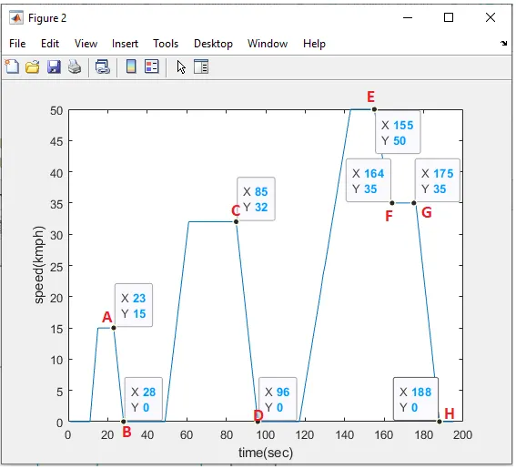
The braking energy is calculated at redardation. The retardation is occured ar Ato B, C to D, E to F and G to H. The speeds at these points are metioned in the figure.

Assume M=1000kg

Eab=0.5*M*(v2-v1)^2*(t2-t1)

= 0.5*1000*(15)^2*(5)

=562kJ

Ecd=1936kJ

Eef=607.5kJ

Egh=2950.5kJ

Total braking energy = Eab+Ecd+Eef+Egh

= 562+1936+607.5+2950.5

= 6056kJ.

2.

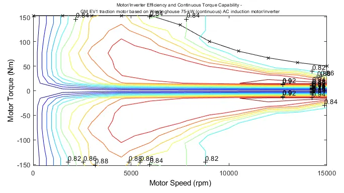
FIG: Torque Speed Characteristics
The figure represents forward motoring (positive torque and speed) and forward braking (negative torque and positive speed).
We know that torque of the induction motor is in inverse proportional to the square of the rotor speed. So at higher speed the
torque will be less. That’s why at high speed electric motor cannot produce braking torque similar to starting.

How electric and mechanical brakes are coordinated?
The electric motor must be controlled to produce the proper amount of braking force to recover as much braking energy as
possible and at the same time, the total braking force must be sufficient to meet vehicle deceleration commanded by thedriver. For meeting the sufficient braking in EV vehicle we use brake control strategies.

Series brake control: Here mechanical brake and electrical brake is done one after another.

Parallel brake control: Here both brakes are applied simultaneously.

We need both mechanical and electrical braking system. In emergency braking or parking brake we needed mechanical braking.
Mechanical brake: It is nothing but friction brakes used in vehicle to slow down the vehicle. The most common type of brakes
are drum brake and disc brake.

Electrical braking: It is used to reduce the speed of the motor depending upon the flux and torque. This kind of braking can be
done in different methods.
Plugging type braking
Dynamic braking
Regenerative braking

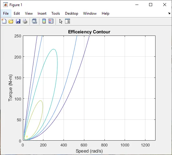
3.Make a MATLAB program which plots contour of given motor speed, torque and efficiency values. Attach the code as a .m file attach a screenshot of all the plots

The relation between motor speed, torque and efficiency values are given as follows

Power= Speed*Torque

Copper loss,

Iron loss,

Windage loss,

Constant loss, C

Where,

ω – Speed (rad/s)

T – Toque (Nm)

cu = kc ⋅ T^ 2

I = ki ⋅ ω

W = kw ⋅ ω^3

The kc,ki and kw are assumed for calculating the contour

clc
clear all
close all
%Program for efficiency contour plot
s=linspace(0,1300); %Motor Speed(rad/sec)
t=linspace(0,250); %Torque(Nm)
kc=0.23; %Copper loss constant
ki=0.06; %Iron loss constant 
kw=0.0002; %Windage loss constant
c=5; %Constant
[x,y]=meshgrid(s,t);
output_power= (x.*y); %Power = speed * torque
cu=kc.*(y.^2); %Copper loss= kc*torque^2
I=ki.*x; %Iron loss= speed*ki
w=kw.*(x.^3); %Windage loss= kw*speed^3
input_power=output_power+cu+I+w+c; %Input power= Output power+Losses
z=output_power./input_power; %Efficiency
%Mapping of efficiency point
v=[0.70,0.75,0.80,0.84,0.90,0.95];
contour(x,y,z,v)
grid on;
title('Efficeiency Contour')
xlabel('Speed (rad/s)');
ylabel('Torque (N-m)');