Steady and Unsteady 2D heat conduction
Steady State Analysis and Transient State analysis
In this we solve the the 2D heat conduction equation by using point iterative methods like Jacobi, Gauss siedel
and Sucessive Over-Relaxation.
Given:
The Boundary Conditions for the problem.
| Top Boundary | 600K |
| Bottom Boundary | 900K |
| left boundary | 400K |
| Right Boundary | 800K |
The error criteria is 1e-4
To solve the equation:
we need to solve 2D heat conduction for both steady and unsteady equations by implicit and explicit schemes:
| steady state | Transient state | |
| Implicit | Implicit | Explicit |
| Jacobi | Jacobi | ------------------ |
| Gauss siedel | Gauss Siedel | ------------------ |
| Sucessive Over-Relaxation | Sucessive Over-Relaxation | ------------------ |
Solution:
Steady State analysis:
The 2D heat conduction equation
`frac{partial^2T}{delx^2}+frac{partial^2T}{dely^2}=0`
T=temperature in Kelvin
t=time
Descritization of the equation is done:
with respect to x:
`frac{T(i-1,j) -2T(i,j)+T(i+1,j)}{Deltax^2}`
with respect to y:
`frac{T(i,j-1) -2T(i,j)+T(i,j+1)}{Deltay^2}`
so final descitized equation
`T(i,j)=(1/k)[frac{T(i-1,j) +T(i+1,j)}{Deltax^2}+frac{T(i-1,j) +T(i+1,j)}{Deltay^2}]`
where `k=frac{2(Deltax^2+Deltay^2)}{Deltax^2Deltay^2}`
nwe solve for different iterative solvers like Jacobi, Gauss siedel and Suceessive over relaxation for implicit schemes
steady state Implicit schemes:
Code for steady state Jacobi:
close all
clear all
clc

%inputs
n=10;
x=linspace(0,1,n);
y=linspace(0,1,n);
dx=dy=0.1;
k=(2*(dx^2+dy^2))/(dx^2*dy^2);
T=ones(n)

%boundary conditions
T(1,1:n)=600 %top bc
T(n,1:n)=900 %bottom bc
T(1:n,1)=400%left bc
T(1:n,n)=800%right bc
Told=T;
iterative_solver=1
tol=1e-4;
error=1;

if iterative_solver==1
  jacobi_iter=1
  while error>tol
    %Told=T
    for i=2:n-1;
     for j=2:n-1;
      T(i,j)=k^-1*(((Told(i-1,j)+Told(i+1,j))/dx^2)+((Told(i,j-1)+Told(i,j+1))/dy^2));
    end
  end
  error=max(max(abs(Told-T)));
  Told=T;
  jacobi_iter=jacobi_iter+1;

endwhile
figure(1)
contourf(T);
colormap('jet');
colorbar;
axis ij;
xlabel('x axis')
ylabel('y axis')
title_text1=sprintf('steady state SOR');
title_text2=sprintf('iteration number=%d',jacobi_iter);
title({title_text1,title_text2});
endif
Code for steady state Gauss siedel
close all
clear all
clc

%inputs
n=10;
x=linspace(0,1,n);
y=linspace(0,1,n);
dx=dy=0.1;
k=(2*(dx^2+dy^2))/(dx^2*dy^2);
T=ones(n)

%boundary conditions
T(1,1:n)=600 %top bc
T(n,1:n)=900 %bottom bc
T(1:n,1)=400%left bc
T(1:n,n)=800%right bc
Told=T;
iterative_solver=1
tolerance=1e-4;
error2=1;

if iterative_solver==1
  gs_iter=1;
  while error2>tolerance
    %Told=T
    for i=2:n-1;
     for j=2:n-1;
      T(i,j)=k^-1*(((T(i-1,j)+T(i+1,j))/dx^2)+((T(i,j-1)+T(i,j+1))/dy^2));
    end
  end
  error2=max(max(abs(Told-T)));
  Told=T;
  gs_iter=gs_iter+1;

endwhile
figure(2)
contourf(T);
colormap('jet');
colorbar;
axis ij;
xlabel('x axis')
ylabel('y axis')
title_text1=sprintf('steady state Gauss seidel');
title_text2=sprintf('iteration number=%d',gs_iter);
title({title_text1,title_text2});
end
code for steady state Successive over-relaxation:
close all
clear all
clc

%inputs
n=10;
x=linspace(0,1,n);
y=linspace(0,1,n);
dx=dy=0.1;
k=(2*(dx^2+dy^2))/(dx^2*dy^2);
T=ones(n)

%boundary conditions
T(1,1:n)=600 %top bc
T(n,1:n)=900 %bottom bc
T(1:n,1)=400%left bc
T(1:n,n)=800%right bc
Told=T;
Tinitial = T;
w=1.4
iterative_solver=1
tol=1e-4;
error3=1;
error3 = 1;
Told = Tinitial;

if iterative_solver==1
      sor_iter=1;
     while error3>tol
    %Told=T
     for i=2:n-1;
     for j=2:n-1;
      T(i,j)=(1-w)*Told(i,j) + (w*0.25*(T(i-1,j)+Told(i+1,j)+T(i,j-1)+Told(i,j+1)));
      end
  end
  error3=max(max(abs(Told-T)))
  Told=T;
  sor_iter=sor_iter+1;
    endwhile

figure(1)
contourf(T);
colormap('jet');
colorbar;
axis ij;
xlabel('x axis')
ylabel('y axis')
title_text1=sprintf('steady state SOR');
title_text2=sprintf('iteration number=%d',sor_iter);
title({title_text1,title_text2});
pause(0.3);

endif
output plot:(implicit schmes)
steady state jacobi steady state gauss sieldel
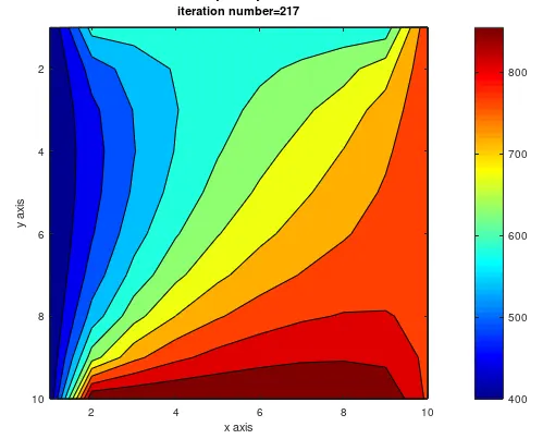
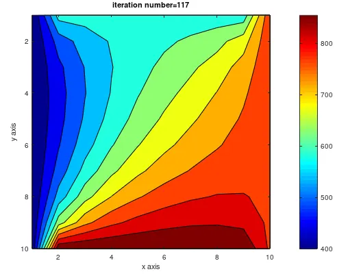
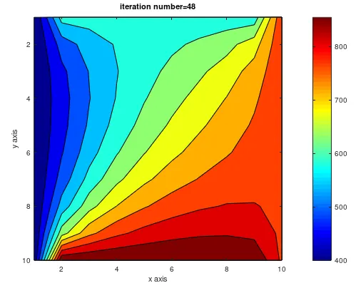
steady state SOR
------------------------------------------------------------------------------------------------------------------------------------------------------------------
------------------------------------------------------------------------------------------------------------------------------------------------------------------
------------------------------------------------------------------------------------------------------------------------------------------------------------------
Transient State analysis:
The 2D heat conduction equation with time
`frac{delT}{delt}=alpha(frac{partial^2T}{delx^2}+frac{partial^2T}{dely^2})`
T=temperature in Kelvin
t=time
descreitizing will give us
`T(i,j)=Told(i,j)+k1[Told(i-1,j)-2Told(i,j)+Told(i+1,j)]+k2[Told(i,j-1)-2Told(i,j)+Told(i,j+1)]`
where `k1=alphafrac{dt}{dx^2}`
`k2=alphafrac{dt}{dy^2}`
first we code for a implicit schemes for jacobi, gauss siedel and SOR:
Implicit scheme:
code for transient jacobi:
clear all
close all
clc
%inputs
n=10;

x=linspace(0,1,n);
y=linspace(0,1,n);
dx=dy=0.1;
dt=30;
alpha=1.4;
k1=(alpha*dt)/dx^2;
k2=(alpha*dt)/dy^2;
term1=(1/(2*k1+2*k2));
term2=k1*term1;
term3=k2*term1;
T=ones(n)

%boundary conditions
T(1,1:n)=600 %top bc
T(n,1:n)=900 %bottom bc
T(1:n,1)=400%left bc
T(1:n,n)=800%right bc
Told=T;
T_prev=Told;
iterative_solver=1
tol=1e-4;
error5=1;


if iterative_solver==1
    jacobi_iter_transient=1
  while error5>tol
    %Told=T
    for i=2:n-1;
     for j=2:n-1;
     H=(Told(i-1,j)+Told(i+1,j));
     V=(Told(i,j-1)+Told(i,j+1));
     T(i,j)=(term1*T_prev(i,j)) + (term2*H) + (term3*V);

    end
  end
  error5=max(max(abs(Told-T)));
  Told=T;
  jacobi_iter_transient=jacobi_iter_transient+1;

  endwhile

figure(1)
contourf(T);
colormap('jet');
colorbar;
axis ij;
xlabel('x axis')
ylabel('y axis')
title_text1=sprintf('Transient implicit jacobi')
title_text2=sprintf('iteration number=%d',jacobi_iter_transient);
title({title_text1,title_text2})
pause(0.3)
endif
code for Transient Gauss sieldel
clear all
close all
clc
%inputs
n=10;

x=linspace(0,1,n);
y=linspace(0,1,n);
dx=dy=0.1;
dt=30;
alpha=1.4;
k1=(alpha*dt)/dx^2;
k2=(alpha*dt)/dy^2;
term1=(1/(2*k1+2*k2));
term2=k1*term1;
term3=k2*term1;
T=ones(n)

%boundary conditions
T(1,1:n)=600 %top bc
T(n,1:n)=900 %bottom bc
T(1:n,1)=400%left bc
T(1:n,n)=800%right bc
Told=T;
T_prev=Told;
iterative_solver=1
tol=1e-4;
error6=1;


if iterative_solver==1
    gs_iter_transient=1
  while error6>tol
    %Told=T
    for i=2:n-1;
     for j=2:n-1;
         H=(T(i-1,j)+Told(i+1,j));
         V=(T(i,j-1)+Told(i,j+1));
         T(i,j)=(term1*T_prev(i,j)) + (term2*H) + (term3*V);

    end
  end
  error6=max(max(abs(Told-T)));
  Told=T;
  gs_iter_transient=gs_iter_transient+1;

  endwhile

figure(1)
contourf(T);
colormap('jet');
colorbar;
axis ij;
xlabel('x axis')
ylabel('y axis')
title_text1=sprintf('Transient implicit gauss siedel')
title_text2=sprintf('iteration number=%d',gs_iter_transient);
title({title_text1,title_text2})
pause(0.3)
endif
code for transient SOR:
clear all
close all
clc
%inputs
n=10;
w=1.3;
x=linspace(0,1,n);
y=linspace(0,1,n);
dx=dy=0.1;
dt=30;
alpha=1.4;
k1=(alpha*dt)/dx^2;
k2=(alpha*dt)/dy^2;
term1=(1/(2*k1+2*k2));
term2=k1*term1;
term3=k2*term1;
T=ones(n)

%boundary conditions
T(1,1:n)=600 %top bc
T(n,1:n)=900 %bottom bc
T(1:n,1)=400%left bc
T(1:n,n)=800%right bc
Told=T;
T_prev=Told;
iterative_solver=1
tol=1e-4;
error7=1;

if iterative_solver==1
    sor_iter_transient=1
  while error7>tol
    %Told=T
    for i=2:n-1;
     for j=2:n-1;
         H=(T(i-1,j)+Told(i+1,j));
         V=(T(i,j-1)+Told(i,j+1));
         T(i,j)=(1-w)*Told(i,j) + w*((term1*T_prev(i,j)) + (term2*H) + (term3*V));
       end
  end
  error7=max(max(abs(Told-T)));
  Told=T;
  sor_iter_transient=sor_iter_transient+1;
  endwhile

figure(1)
contourf(T);
colormap('jet');
colorbar;
axis ij;
xlabel('x axis')
ylabel('y axis')
title_text1=sprintf('Transient implicit SOR')
title_text2=sprintf('iteration number=%d',sor_iter_transient);
title({title_text1,title_text2})
pause(0.3)
endif
Explicit - Transient:
code for Transient explicit:
clear all
close all
clc
%inputs
n=10;
x=linspace(0,1,n);
y=linspace(0,1,n);
dx=dy=0.1;
dt=30;
alpha=2.2e-5;
k1=(alpha*dt)/dx^2;
k2=(alpha*dt)/dy^2;
T=ones(n)

%boundary conditions
T(1,1:n)=600 %top bc
T(n,1:n)=900 %bottom bc
T(1:n,1)=400%left bc
T(1:n,n)=800%right bc
Told=T;
iterative_solver=1
tol=1e-4;
error4=1;

if iterative_solver==1
    iter=1
  while error4>tol
    %Told=T
    for i=2:n-1;
     for j=2:n-1;
     term1=Told(i,j);
     term2=k1*(Told(i-1,j) - 2*Told(i,j)+ Told(i+1,j));
     term3=k2*(Told(i,j-1) - 2*Told(i,j)+ Told(i,j+1));
     T(i,j)=(term1+term2+term3);
    end
  end
  error4=max(max(abs(Told-T)));
  Told=T;
  iter=iter+1;
  endwhile

figure(1)
contourf(T);
colormap('jet');
colorbar;
axis ij;
xlabel('x axis')
ylabel('y axis')
title_text1=sprintf('Transient explicit')
title_text2=sprintf('iteration number=%d',iter);
title({title_text1,title_text2})
pause(0.3)
endif
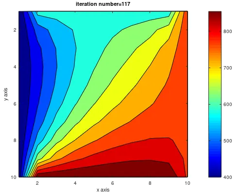
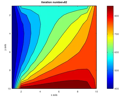
Output plot for transient implicit scheme:
transient jacobi transient gauss siedel
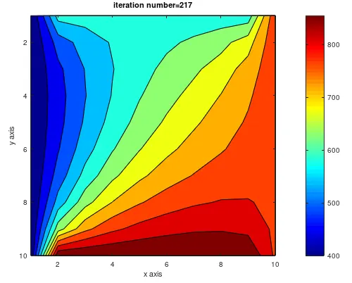
transient SOR
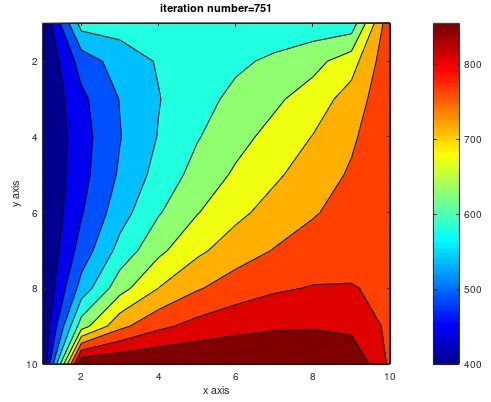
Output plot for transient explicit scheme:
Explanation for the code :
- First we declare the nodes,x axis and y axis along with dx and dy.
- Make a matrix for Temp with 10rows and 10 columns
- Declare the boundary conditions.
- set Told to T and Tinitial to T to avoid confusion and store the old values.
- Set the iterative solver and give values for error and tolerance.
- start an if loop for solver.
- start a while loop for error>tolerance.
- start a for loop within the while loop for iterating values of i,j in the Temperature descretized 2d conduction equation.
- After ending the for loop calculate the error that is maximum of absolute of Told-T and store Told in T.
- Increase the loop counter by 1 and end while loop
- Plot the contour of Temperature T and end if loop.
Explanation for plots/results :
- The plots are made for implicit schemes by using iterative solvers like jacobi,gauss siedel and Successive over-Relaxation.
- In this the steady state 2d conduction equation is descretized to be solved.
- The iterations taken by the jacobi method is more than that of gauss siedel and SOR
- Jacobi iteration>Gauss siedel>SOR
- By this we can interpret that jacobi takes more time and steps to reach solution or converge at slower rate.
- we can see that the SOR takes very less iterations to converge.
- so convergence rate is Jacobi<gauss siedel<SOR
- The SOR converges faster due to the omega which is a relaxation parameter and when used properly can help to converge at good rates irrespective of schemes used.
- The convergence iteration:for implict schemes steady state SOR does in 48 iteration and transient sor in 68
- the convergance rate by explicit take more iteration than any other method.
- The relaxation parameter omega(w)can be computed and about 1.2 to 1.4 then the solution converges faster and as we increases omega it again sweep back to more iterations so the optimum value is disturbed.
- So we can say that value of relaxation factor is a key aspect to less iteration.
,