Week 7 - Simulation of a 1D Super-sonic nozzle flow simulation using Macormack Method

Aim :To simulate the isentropic flow through a quasi 1D subsonic_supersonic nozzle by Macormack's technique.

Objectives:

• Steady-state distribution of primitive variables inside the nozzle.
• Time-wise variation of the primitive variables
• Variation of Mass flow rate distribution inside the nozzle at different time steps during the time-marching process
• Comparison of Normalized mass flow rate distributions of both forms

Theory :

we consider steady ,isentropic flow through the convergent- divergent nozzle in the fig

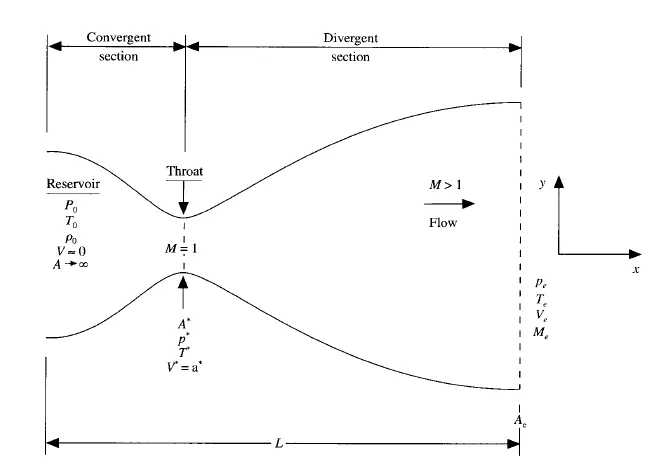
The flow at the inlet of the nozzle comes from a reservoir where pressure and temperature are denoted by `punderseto` and `Tunderseto` respectively. The cross sectional area of the reservoir is large and hence the velocity is very small and V tends to zero. The flow expands isentropically to the supersonic speeds ,where the pressure ,temperature,velocity and mach number at the exit are `pundersete`,`Tundersete`,`Vundersete`,`Mundersete`.The flow is locally subsonic at convergent section of the nozzle and locally supersonic at the divergent section of the nozzle.

The sonic flow is M=1 at the throat, M<1 at the entrance and M>1 at the exit.

At sonic value flow V=V*=a*

Area of sonic throat A=A*

in reality the flow is in 2d but we consider only the 1d i.e in x axis so the flow is defined as Quasi 1-d flow.

Governing Equations:

Continuity equation:

`rhounderset1``Vunderset1``Aunderset1`= `rhounderset2``Vunderset2``Aunderset2`

Momentum equation:

`punderset1``Aunderset1` + `rhounderset1``V^2underset1``Aunderset1` + `int_(A1)^(A2) pdA` = `punderset2``Aunderset2` + `rhounderset2``V^2underset2``Aunderset2`

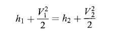
Energy equation:

Conservation and Non-conservation form:

Both Conservative and Non-Conserative forms are analytically equal but the results vary a bit in different problems in cfd.

in general terms if the control volume is fixed and the fluid is moving across the CV then it is conservation form. And if the Control volume is moving with the fluid and the fluid remain inside the volume then its is a non-conservation form.

Initial condition will be different for both conservation and non conservation forms and both the solutions reach steady state after a certain amount of time and it majorly depends upon the CFL stability criteria.

Non dimensional quantities:

`T'=frac{T}{To}` -----non dimensionless temperature

`rho'= frac{rho}{rhoo}`------non dimensionless density

`x'=frac{x}{L}`-----------dimensionless length

`ao= sqrt(gamma RTunderseto`--------speed of sound in the reservoir

`V'=frac{V}{ao}`-------------------dimensionless velocity

`t'= frac{t}{L/{ao}}`--------------dimensionless time

`A' = frac{A}{A*}`------------------dimensionless area

`frac{T}{To}=(1+frac{gamma-1}{2}M^2)^-1`

`frac{rho}{rhoo}=(1+frac{gamma-1}{2}M^2)^(-1/(gamma-1))`

`frac{p}{po}=(1+frac{gamma-1}{2}M^2)^(-1/(gamma-1))`

GOVERNING EQUATIONS

We fundamentally follow three principles of physics:

• Mass conservation
• momentum conservation ;which is newtons second law of motion
• Energy conservation

Derivation:

consider a small strip of area dx on the control volume of the nozzle where inlet and exit is varied by a factor of dx or change in primitive terms.

consider an intergal form of continuity equation

`frac{del}{delt} intintint_VrhodV+intint_SrhoVds=0`-----------(1)

Volume Intergral:

`frac{del}{delt}intintint_VrhodV = del/(delt)(rhoAdx)`-----------(2)

Surface Integral:

`intint_SrhoVds=-rhoVA+(rho+drho)(V+dV)(A+dA)`

`intint_SrhoVds = d(rhoAV)`------------------------------------(3)

put eqn 2 and 3 in 1 we get the continuity equation

`del/(delt)(rhoAdx)+del(rhoAV)`

divide by dx

Continuity equation:

`del/(delt)(rhoA)+del/(delx)(rhoAV)`---------------------continuity equation in conservation form

Now we need to find the integral form of momentum equation:

`del/(delt)intintint_V(rhou)dV+intint_S(rhouv)ds = -intint_s(pds)`--------------(4)

`del/(delt)intintint_V(rhou)dV= del/(delt)(rhoVAdx)`------------------------------(5)

`intint_S(rhouv)ds = -rhoV^2A + (rho+drho)(V+dV)^2(A+dA)`----------------(6)

`intint_s(pds)= -pA+(p+dp)(A+dA)-2p((dA)/2)`---------------------------------(7)

put eqn 5,6,7 in eq 4 we get

Momentun Equation

`del/(delt)(rhoVA)+del/(delx)(rhoV^2A)=-Afrac{delp}{delx}`---------momentum equation in non conservation form

Now we need to find the integral form of Energy equation:

`del/(delt)intintint_Vrho(e+V^2/2)dV+intint_Srho(e+V^2/2)V.dS = -intint_S(pV)dS`

`del/(delt)[rho(e+V^2/2)Adx]-rho(e+V^2/2)VA+(rho+drho)[e+de+(V+dV)^2/2](V+dV)(A+dA)=-[-pVA+(p+dp)(V+dV)(A+dA)-]2(pV(dA)/2)`

`del/(delt)[rho(e+V^2/2)Adx]+d[rho(e+V^2/2)Adx] = -d(pAV)`---------energy equation

divide by dx

`del/(delt)[rho(e+V^2/2)A]+del/(delx)[rhoV(e+V^2/2)Adx] = -d(pAV)`---------energy equation in conservation form

Non-conservation form:

Conservation form can be multiplied by V to get non-conservation forms

---continuity equation:

`frac{delrho'}{delt'}=-rho'frac{delV}{delx'}-rho'V'frac{del(lnA')}{delx'}-V'frac{delrho'}{delx'}`

---Momentum equatuion:

`frac{delV'}{delt'} =-V'frac{delV'}{delx'}-(1/gamma)(frac{delT'}{delx"}+frac{T'}{rho'}frac{delrho'}{delx'})`

---- Energy equation:

`frac{delT'}{delt'} = -V'frac{delT'}{delx'}-(gamma-1)[frac{delV'}{delx"}+V'frac{del(ln A')}{delx'}]`

Conservation form:

to find the solution in conservation forn we need to make a solution vector U, the flux vector F and the source term J.This is because if we write equation in primitive variables then instabilities

develop during the course of time marching solution. For the present problem instabilities develop in the subsonic section which can cause the solution to blow up after 300 time steps.

`U1=rho'A'`

`U2=rho'A'V'`

`U3=rho'((e')/(gamma-1)+(gamma/2)V'^2)A'`

`F1= rho'A'V'`

`F2=rho'A'V' + (1/gamma)p'A'`

`F3=rho'((e')/(gamma-1)+(gamma/2)V'^2)V'A'+p'A'V'`

`J2=(1/gamma)p'((delA')/(delx'))`

`frac{delU1}{delt'} = -frac{delF1}{delx'}`----------------------continuity eqn in conservation form interms of solution and flux vector terms

`frac{delU2}{delt'} = -frac{delF2}{delx'}+J2` ------------------momentum eqn in conservation form interms of solution and flux vector terms

`frac{delU3}{delt'} = -frac{delF3}{delx'}`----------------------Energy eqn in conservation form interms of solution and flux vector terms

pure form of flux terms:

F1=U2;

`F2=frac{U2^2}{U1}+(gamma-1)/gamma(U3-gamma/2(frac{U2^2}{U1}))`

`F3=(gammaU2U3)/(U1)-(gamma(gamma-1))/2((U2^3)/(U1^2))`

`J2=(gamma-1)/gamma(U3-gamma/2(U2^2)/(U1))(del(lnA'))/(delx')`

CFL criteria for finding dt:

`Deltat=(lamdaDeltax)/(V+a)`

`lamda=`courant number

`Deltax`=step size

`Deltat`=Time step

V=velocity

a= speed of sound

Macormacks Technique:

Its an explicit finite difference technique which is second order accurate in both space and time

Non conservative approach:

In Macormack technique we split time marching in to two phases which are predictor phase and actual phase

Initial conditions:

`rho =1-0.3146x`

`T=1-0.2314x`

V=(0.1+1.0x)T^(0.5)

A=1+2.2(x=+-1.5) ^2 `0<=x<=3`

discretization:

predictor step:

The space terms will be forward differenced.

`(delrho)/(delti)=-rhoi[(V(i+1)-V(i))/(Deltax)]-rhoiVi[(lnA(i+1)-lnA(i))/(Deltax)]-Vi[(rho(i+1)-rho(i))/(Deltax)]`

`(delV)/(delti,p)=-Vi[(V(i+1)-V(i))/(Deltax)]-(1/gamma)((T(i+1)-T(i))/(Deltax)+((Ti)/(rhoi)(V(i+1)-V(i))/(Deltax))`

`(delT)/(delti,p)=-Vi[(T(i+1)-T(i))/(Deltax)]-(gamma-1)T(i)((V(i+1)-V(i))/(Deltax)+Vi(lnA(i+1)-lnA(i))/(Deltax))`

Solution Update:

`rhoi^(updated)=rhoi^(Initial)+(delrho)/(delti,p)dt`

`Vi^(updated)=Vi^(Initial)+(delV)/(delti,p)dt`

`Ti^(updated)=Ti^(Initial)+(delT)/(delti,p)dt`

corrector step

The space terms are backward differenced

`(delrho)/(delti,c)=-rhoi[(V(i)-V(i-1))/(Deltax)]-rhoiVi[(lnA(i)-lnA(i-1))/(Deltax)]-Vi[(rho(i)-rho(i-1))/(Deltax)]`

`(delV)/(delti,c)=-Vi[(V(i)-V(i-1))/(Deltax)]-(1/gamma)((T(i)-T(i-1))/(Deltax)+((Ti)/(rhoi)(V(i)-V(i-1))/(Deltax))`

`(delT)/(delti,c)=-Vi[(T(i)-T(i-1))/(Deltax)]-(gamma-1)T(i)((V(i)-V(i-1))/(Deltax)+Vi(lnA(i)-lnA(i-1))/(Deltax))`

Average time derivative:

`(delrho)/(delt,avg)=0.5((delrho)/(delti,p)+(delrho)/(delti,c))`

`(delV)/(delt,avg)=0.5((delV)/(delti,p)+(delV)/(delti,c))`

`(delT)/(delt,avg)=0.5((delT)/(delti,p)+(delT)/(delti,c))`

Updated final solution:

`rhoi^(2^(nd)update)=rhoi^(Initial)+(delrho)/(delti,avg)dt`

`Vi^(2^(nd)update)=Vi^(Initial)+(delV)/(delti,avg)dt`

`Ti^(2^(nd)update)=Ti^(Initial)+(delT)/(delti,avg)dt`

Conservation Approach:

initial profiles:

`rho=1; 0<=x<=0.5`

`rho=1-0.366(x-0.5); 0.5<=x<=1.5`

`rho=0.634-0.3879(x-1.5); 1.5<=x<=3`

`T=1 ; 0<=x<=0.5`

`rho=1-0.167(x-0.5); 0.5<=x<=1.5`

`rho=0.833-0.3507(x-1.5); 1.5<=x<=3`

area `A=1+2.2(x-1.5)^2;0<=x<=3`

Boundary condition:

U1=fixed value of 1;

`U2(i=1)=2U2(i=2)-U2(i=3)`-----------------------------internal grid point

for end boundary points

`U1(n)=2(U1)(n-1)-(U1)(n-2)`

`U2(n)=2(U2)(n-1)-(U2)(n-2)`

`U3(n)=2(U3)(n-1)-(U3)(n-2)`

Macormacks technique on conservation form:

predictor step:

`(delU1)/(deltp)=-frac{F1(i+1)-F1(i)}{Deltax}`

`(delU2)/(deltp)=-frac{F2(i+1)-F2(i)}{Deltax}+J2(i)`

`(delU3)/(deltp)=-frac{F3(i+1)-F3(i)}{Deltax}`

updated values of intermediate step

`overlineU1=U1+(delU1)/(deltp)`

`overlineU2=U2+(delU2)/(deltp)`

`overlineU3=U3+(delU3)/(deltp)`

corrector step

`(delU1)/(deltc)=-frac{overlineF1(i)-overlineF1(i-1)}{Deltax}`

`(delU2)/(deltc)=-frac{overlineF2(i)-overlineF2(i-1)}{Deltax}+overlineJ2(i)`

`(delU3)/(deltc)=-frac{overlineF3(i)-overlineF3(i-1)}{Deltax}`

Final solution update

`U1^(n+1)=U1^(n)+frac{(delU1)/(deltp)+(delU1)/(deltc)}{2}`

`U2^(n+1)=U2^(n)+frac{(delU2)/(deltp)+(delU2)/(deltc)}{2}`

`U3^(n+1)=U3^(n)+frac{(delU3)/(deltp)+(delU3)/(deltc)}{2}`

Code for macormack method implemented for both non-conservation form and conservation form

Main code:

clear all 
close all
clc
%--------------------------------------------------------------------------------------------------------
%inputs
n=31;
L=3;
x=linspace(0,L,n);
dx=x(2)-x(1);
gamma=1.4;
nt=700;
massflowrate=zeros(30);
throat=find(x==1.500) ;%throat section at x=1.5
a=1+2.2*(x-1.5).^2;%area
c=0.5;

%%Non conservative form solution
tic;
[M,massflowrate,v,t,p,rho,t_throat,p_throat,rho_throat,M_throat]=one_d_supersonic_non_conserve(x,dx,n,c,a,nt,gamma,throat)
time_taken_non_cons=toc;

%%time variation of primitive variables(non conserve)
time_variation= figure(2);
subplot(4,1,1)
plot(rho_throat,'-b')
title('time wise variation of primitive variables')
legend('density');
ylabel('rho/rho_o');
axis([0 700 0 1.3]);
grid minor;

subplot(4,1,2)
plot(t_throat,'-r')
legend('temperature');
ylabel('t/t_o');
axis([0 700 0.6 1]);
grid minor;

subplot(4,1,3)
plot(p_throat,'-g')
legend('pressure');
ylabel('p/p_o');
axis([0 700 0.4 1.1]);
grid minor;

subplot(4,1,4)
plot(M_throat,'-c')
legend('mach');
ylabel('mach');
axis([0 700 0.6 1.4]);
grid minor;

%non conservation steady state distribution of primitve variables
steady_state=figure(3);
subplot(4,1,1)
plot(x,M,'-b');
title('steady state non-conservative');
ylabel('M');
legend('mach number');
grid minor;

subplot(4,1,2)
plot(x,p,'-g');
ylabel('p/p0');
legend('pressure ratio');
grid minor;

subplot(4,1,3)
plot(x,rho,'-c');
ylabel('rho/rho_0');
legend('density ratio');
grid minor;

subplot(4,1,4)
plot(x,t,'-r');
ylabel('t/t0');
legend('temperature ratio');
grid minor;
% %------------------------------------------------------------------------------------------------
%%conservative form solution
tic;
[M_c,massflowrate_c,v,T,p,rho,T_throat_c,p_throat_c,rho_throat_c,M_throat_c]=one_d_super_conserve(x,n,dx,throat)
time_taken_cons=toc;

time_variation_con=figure(6);%conserve

subplot(4,1,1)
plot(rho_throat_c,'-b')
title('time wise variation of primitive variables,conservative')
legend('density');
ylabel('rho/rho_o');
%axis([0 700 0 1.3]);
grid minor;

subplot(4,1,2)
plot(T_throat_c,'-r')
legend('temperature');
ylabel('t/t_o');
%axis([0 700 0.6 1]);
grid minor;

subplot(4,1,3)
plot(p_throat_c,'-g')
legend('pressure');
ylabel('p/p_o');
%axis([0 700 0.4 1.1]);
grid minor;

subplot(4,1,4)
plot(M_throat_c,'-b')
legend('mach');
ylabel('mach');
%axis([0 700 0.6 1.4]);
grid minor;

%%primitive variables conservation steady state
steady_state=figure(7);
subplot(4,1,1)
plot(x,M_c,'-b');
title('steady state conservative');
ylabel('M');
legend('mach number');
grid minor;

subplot(4,1,2)
plot(x,p,'-g');
ylabel('p/p0');
legend('pressure ratio');
grid minor;

subplot(4,1,3)
plot(x,rho,'-c');
ylabel('rho/rho_0');
legend('density ratio');
grid minor;

subplot(4,1,4)
plot(x,T,'-r');
ylabel('t/t0');
legend('temperature ratio');
grid minor;

%-----------------------------------------------------------------
%%comparision of mass flow by conservative and non-conservative
mfr_comparision=figure(8)
hold on;
plot(x,massflowrate,'-b');
plot(x,massflowrate_c,'-g');
legend('non-conservative','conservative');
grid minor;
xlabel('x/L');
ylabel('rhova/rho_0a_oA*');

Non-conservation Form function:

function[M,massflowrate,v,t,p,rho,t_throat,p_throat,rho_throat,M_throat]=one_d_supersonic_non_conserve(x,dx,n,c,a,nt,gamma,throat)

%calculate initial profile
rho=1-0.3146*x;
t=1-0.2314*x;  %(t=temp)
v=(0.1+1.09*x).*t.^0.5;
massflowrate=zeros(30);
%cfl no time step control in project.

%outer loop k=time
for k=1:nt
    rho_old=rho;
    v_old=v;
    t_old=t;
    dt=min(c.*dx./(sqrt(t)+v));

    %prediction
    %method--------------------------------------------------------------------------
   
    %continuity eqn
    for j=2:n-1
        %drho_dt_p=-rho(j)*(v(j+1)-v(j))/dx-rho(j)*v(j)*(log(a(j+1)-a(j)))/dx-v(j)*(rho(j+1)-rho(j))/dx;
        drhodx=(rho(j+1)-rho(j))/dx;
        dvdx= (v(j+1)-v(j))/dx;
        dtdx=(t(j+1)-t(j))/dx;
        dlogadx = (log(a(j+1))-log(a(j)))/dx;
        
        %continuity eqn
        drho_dt_p(j) = -rho(j)*dvdx - rho(j)*v(j)*dlogadx -  v(j)*drhodx;
        
        %momentum eqn
        dvdt_p(j) = -v(j)*dvdx - (1/gamma)*(dtdx + (t(j)/rho(j))*drhodx);
        
        %energy eqn
        dtdt_p(j) = -v(j)*dtdx - (gamma-1)*t(j)*(dvdx + v(j)*dlogadx);
        
        %solution update
        rho(j) = rho(j) + drho_dt_p(j)*dt;
        v(j) = v(j)+ dvdt_p(j)*dt;
        t(j) = t(j) + dvdt_p(j)*dt;
    end
        
    % corrector step space terms backward differencing
    for j=2:n-1
        %drho_dt_p=-rho(j)*(v(j+1)-v(j))/dx-rho(j)*v(j)*(log(a(j+1)-a(j)))/dx-v(j)*(rho(j+1)-rho(j))/dx;
        drhodx=(rho(j)-rho(j-1))/dx;
        dvdx= (v(j)-v(j-1))/dx;
        dtdx=(t(j)-t(j-1))/dx;
        dlogadx = (log(a(j))-log(a(j-1)))/dx;
        
        %continuity eqn
        drho_dt_c(j) = -rho(j)*dvdx - rho(j)*v(j)*dlogadx -  v(j)*drhodx;
        
        %momentum eqn
        dvdt_c(j) = -v(j)*dvdx - (1/gamma)*(dtdx + (t(j)/rho(j))*drhodx);
        
        %energy eqn
        dtdt_c(j) = -v(j)*dtdx - (gamma-1)*t(j)*(dvdx + v(j)*dlogadx);
        
    end
    
    %compute the avg time derivative
    drhodt = 0.5*(drho_dt_p + drho_dt_c)
    dvdt = 0.5*(dvdt_p + dvdt_c)
    dtdt = 0.5*(dtdt_p + dtdt_c)
      
    for i= 2:n-1
    %final solution update
    rho(i) = rho_old(i) + drhodt(i)*dt;
    v(i) = v_old(i) + dvdt(i)*dt;
    t(i) = t_old(i) + dtdt(i)*dt;
    end
    
    %apply boundary condition\
    %inlet
       v(1)=2*v(2) - v(3);
       rho(1)=1;
       t(1)=1;
        
    %outlet
       v(n) = 2*v(n-1) - v(n-2);
       rho(n) = 2*rho(n-1) - rho(n-2);
       t(n) = 2*t(n-1) - t(n-2);
      %non dimensional variables
       p=rho.*t;
       M = v./t.^(1/2);%mach= v/root(T)
       massflowrate= rho.*a.*v;
       
       %calculation of variables at throat
       t_throat(k)=t(throat);
       p_throat(k)=p(throat);
       rho_throat(k)= rho(throat);
       M_throat(k)=M(throat);
       
       mass=figure(1);
       hold on
       if k==50
           plot(x,massflowrate,'r')
       else if k==100
           plot(x,massflowrate,'g')
           else if k==150
           plot(x,massflowrate,'y')
               else if k==200
           plot(x,massflowrate,'c')
                   else if k==700
                         plot(x,massflowrate,'b')
                          plot(x(end),massflowrate(end),'-');
                            end
                   end
               end
           end
       end
end


title('comparision of non-dimen mass flow rates at diff times');
xlabel('x/L');
ylabel('non dimensional mass flow rhova/rho_0a_oA*');
legend('50dt','100dt','150dt','250dt','500dt');
axis([0 3 0 2.5]);
grid on;
grid minor;

Conservation form function:

function[M_c,massflowrate_c,v,T,p,rho,T_throat_c,p_throat_c,rho_throat_c,M_throat_c]=one_d_super_conserve(x,n,dx,throat)
%--------------------------------------------------------------------------------------------------------
%inputs
gamma=1.4;
nt=700;
massflowrate=zeros(1,length(x));
a=1+2.2*(x-1.5).^2;%area
C=0.5;

%%conservative form solution
tic;
%building initial profile
%area = a
a=1+2.2*(x-1.5).^2;
for i=1:length(x)
    if x(i)<=0.5
        rho(i)=1;
        T(i)=1;
    else if x(i)> 0.5 && x(i)<=1.5
        rho(i)=1-0.366*(x(i)-0.5);
        T(i)=1-0.167*(x(i)-0.5);
        else
        rho(i)=0.634-0.3879*(x(i)-1.5);
        T(i) = 0.833-0.3507*(x(i)-1.5);
            end
        end
    end

%dt=0.0267;
v= 0.59./(rho.*a);
p = rho.*T;

% solution vector U
U1 = rho.*a;
U2 = rho.*a.*v;
U3 = U1.*((T./(gamma-1))+(gamma/2)*v.^2);

%for dt with cfl stability criteria
%dt=min(C.*dx./(sqrt(T)+v));

%outer time loop for k

for k=1:nt
    U1_old=U1;
    U2_old=U2;
    U3_old=U3;
    
%     %adaptive cfl time step
     dt=min(C.*dx./(sqrt(T)+v));
      
    %pure flux terms ;flux vector F
    F1=U2;
    F2= ((U2.^2)./U1) + ((gamma-1)/gamma)*(U3-(0.5*gamma*(U2.^2./U1)));
    F3= ((gamma*U2.*U3)./U1) - (0.5*gamma*(gamma-1)*(U2.^3./U1.^2));
    
    %predictor method step1 forward differencing
    for i = 2:n-1
        %source J2
        J2=(1/gamma).*rho(i).*T(i).*((a(i+1)-a(i))/dx);
        
        %continuity eqnn
        dU1dt_p(i)= -(F1(i+1)-F1(i))/dx;
        %momentum eqnn
        dU2dt_p(i)= -(F2(i+1)-F2(i))/dx + J2;
        %energy eqnn
        dU3dt_p(i)= -(F3(i+1)-F3(i))/dx;
         
        %predicted step update
        U1(i)=U1(i)+ dU1dt_p(i)*dt;
        U2(i)=U2(i)+ dU2dt_p(i)*dt;
        U3(i)=U3(i)+ dU3dt_p(i)*dt;
    end
    %variables
    rho=U1./a;
    T=(gamma-1)*((U3./U1)-(0.5*gamma*v.^2));
    p=rho.*T;
    
    %outer loop flux vector
    F1=U2;
    F2= ((U2.^2)./U1) + ((gamma-1)/gamma)*(U3-(0.5*gamma*(U2.^2./U1)));
    F3= ((gamma*U2.*U3)./U1) - (0.5*gamma*(gamma-1)*(U2.^3./U1.^2));
    
    
    
    %corrector step backward diff
     for i = 2:n-1
        J2=(1/gamma).*rho(i).*T(i).*((a(i)-a(i-1))/dx);
        
        %continuity eqnn
        dU1dt_c(i)= -(F1(i)-F1(i-1))/dx;
        %momentum eqnn
        dU2dt_c(i)= -(F2(i)-F2(i-1))/dx + J2;
        %energy eqnn
        dU3dt_c(i)= -(F3(i)-F3(i-1))/dx;
     end
     
     %avg derivative
     dU1dt = 0.5*(dU1dt_p+dU1dt_c);
     dU2dt = 0.5*(dU2dt_p+dU2dt_c);
     dU3dt = 0.5*(dU3dt_p+dU3dt_c);
     
     %corrected values of new solution vector
     for i=2:n-1
         U1(i)=U1_old(i)+dU1dt(i)*dt;
         U2(i)=U2_old(i)+dU2dt(i)*dt;
         U3(i)=U3_old(i)+dU3dt(i)*dt;
     end

     %boundary condition
     %inlet
        
     U1(1)=rho(1)*a(1);
     U2(1)= 2*U2(2)-U2(3);
     v(1) = U2(1)/U1(1);
     U3(1)= U1(1)*((T(1)/(gamma-1))+(0.5*gamma*v(1)^2));
     
     %outlet 
     U1(n)=2*U1(n-1)-U1(n-2);
     U2(n)=2*U2(n-1)-U2(n-2);
     U3(n)=2*U3(n-1)-U3(n-2);
     
    %primitive variable rho,v,T ,p
    rho=U1./a;
    T=(gamma-1)*((U3./U1)-(0.5*gamma*v.^2));
    p=rho.*T;
    v=U2./U1;   
    

    M_c= v./(T.^(1/2));%mach= v/root(T)
    massflowrate_c= U2;  %mfr
    
    %at throat
          
       
    p_throat_c(k)=  p(throat);
    M_throat_c(k) =  M_c(throat);%mach number
    rho_throat_c(k) = rho(throat);
    T_throat_c(k) = T(throat);
    
     figure(11)
     hold on
     if k==100
     plot(x,massflowrate_c,'c');
     else if k==200
              plot(x,massflowrate_c,'b');
         else if k==700
                  plot(x,massflowrate_c,'g');
             end
         end
     end
          
end
   title('comparision of conservative form non-dimen mass flow rates at diff times');
    xlabel('x/L');
    ylabel('non dimensional mass flow rhova/rho_0a_oA*');
    legend('100dt','200dt','700dt');

RESULTS AND DISCUSSIONS:

Non-conservation form

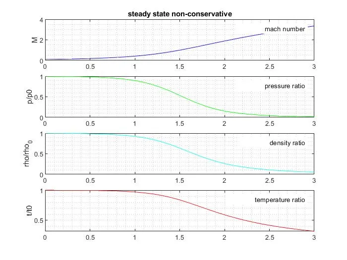
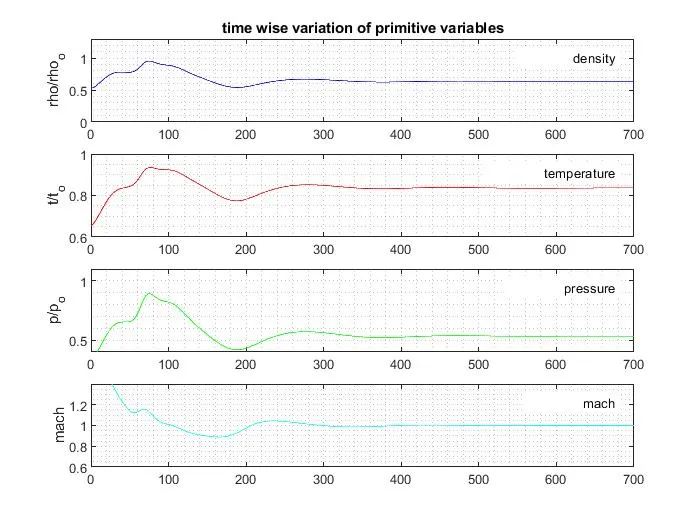
Steady state variation of primitive variables at throat: timewise (transient) variation of primitive variables

Variation of mass flow rate inside the nozzle at different time steps in non-conservation form:

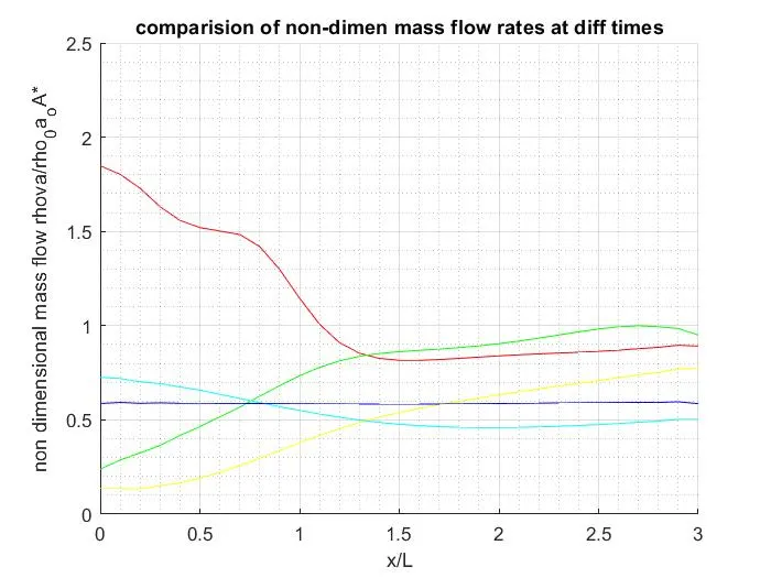
observed inferences from above plots:

• In the steady state plot we can see that mach number has increased from less than zero to the point M>1 and also upto 3 , this shows the variation of mach number from subsonic to supersonic.
• for presssure we can infer that the pressure at reached maximum at the throat which is expected output and later decreased at the exit.
• density also follows the same trend as of pressure.
• temperature variation are seen and can be infered a maximum at throat.
• Transient values for pressure ratio,temperature ratio,density ratio and mach number vary according to a stability criteria and we can see a stable
• time taken for the non conservation part analysis is 6.5367s
• there is pretty good variation of mass flow rate at stating of time marching. As marching proceeds incurence of residuals can be seen till the end state has arrived.

Conservation form

steady state variation of primitive variables Transient state variation of primitve variable (conservation)

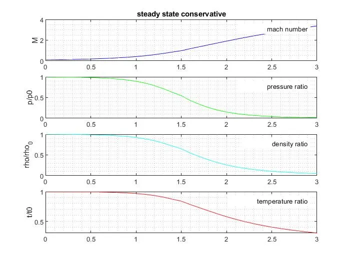
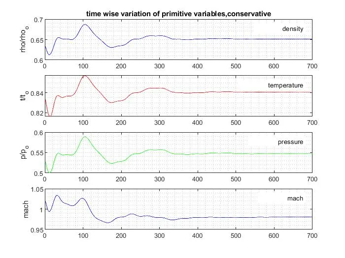
Variation of mass flow rate inside the nozzle at different time steps in Conservation form:

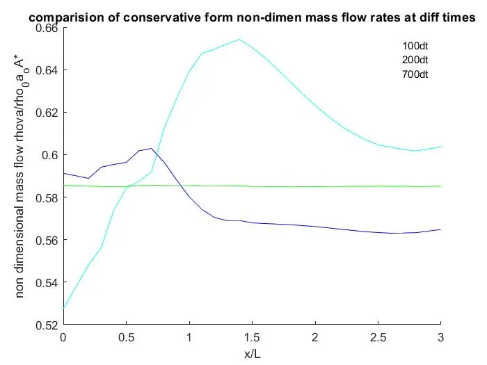
observed inferences from above plots:

• In the steady state plot we can see that mach number has increased from less than zero to the point M>1 and also upto 3 , this shows the variation of mach number from subsonic to supersonic.
• for presssure we can infer that the pressure at reached maximum at the throat which is expected output and later decreased at the exit.
• density also follows the same trend as of pressure.
• temperature variation are seen and can be infered a maximum at throat.
• Transient values for pressure ratio,temperature ratio,density ratio and mach number vary according to a stability criteria and we can see a stable
• time taken for the non conservation part analysis is 4.9905s
• every variable decrease except the mach number at the exit of the nozzle.
• the variation of mass flow rate in conservation form is less over the length of nozzle except for x=1.5 and the variation is not very big but is big in comaprision to throat section.

comaparitive mass flow rates of non-comnservation and conservation forms:

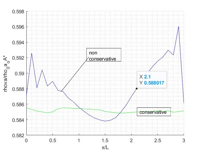
Expalnation for comparision mass flow rate plot:

Its tells about the advantage of conservation approach over the non-conservation one. The conservative mass flow is much better than that of non-conservation as the

conservation form takes primary dependant variables and non-coservation takes secondary dependant variables. so we get a better stable plot for conservation.

Grid independancy test:

The grid dependency test is done to check a scheme can solve faster . By varying the grid size we can check for the accuracy of solution and stability too.

the test is performed on two grid sizes 31 and 61 and been checked fro the stability and accuuracy of the schemes for both consevation and non-conservation.

As in the density ratio we can see a variation of 0.0149 for 31 grid points for non-conservation and conservation forms

As in the temperature ratio we can see a variation of 0.0053 for 31 grid points for non-conservation and conservation forms

As in the pressure ratio we can see a variation of 0.0159 for 31 grid points for non-conservation and conservation forms

As in the mach number we can see a variation of 0.024 for 31 grid points for non-conservation and conservation forms

As in the density ratio we can see a variation of 0.0015 for 61 grid points for non-conservation and conservation forms

As in the temperature ratio we can see a variation of 0.0007 for 61 grid points for non-conservation and conservation forms

As in the pressure ratio we can see a variation of 0.0014 for 61 grid points for non-conservation and conservation forms

As in the mach number we can see a variation of 0.0023 for 61 grid points for non-conservation and conservation forms

Conclusion:

• For mass flow rate comparision we can see that the conservation form produce better results and stable solution.
• upon comparision of both forms we can say there is not much of a difference but the conservation form produce better results and solution time.
• the conservation form is better due to the introduction of secodary variable and the flux vector which reduces the variable count and increases the accuracy
• for grid independence test non conservation takes less time and conservation takes a bit more time , this is due to the introduction of flux variables which require more computing power and time.
• overall both the methods are good and have their own advantages and disadvantages. so we need to choose wisely according the essence of problem to avoid unneccesary blow ups.
• proper schemes are to be chosen so that the order of accuracy is good enough for accurate results.
• courant number is neccesary criteria for time stability of the solution with values from 0.5 to 1 seek better results