Gate Valve Parametric Study
Aim: Perform a parametric study on the gate valve simulation by setting the opening from 10 % to 80%.
Objective:
- Obtain the mass flow rates at the outlet for each design point.
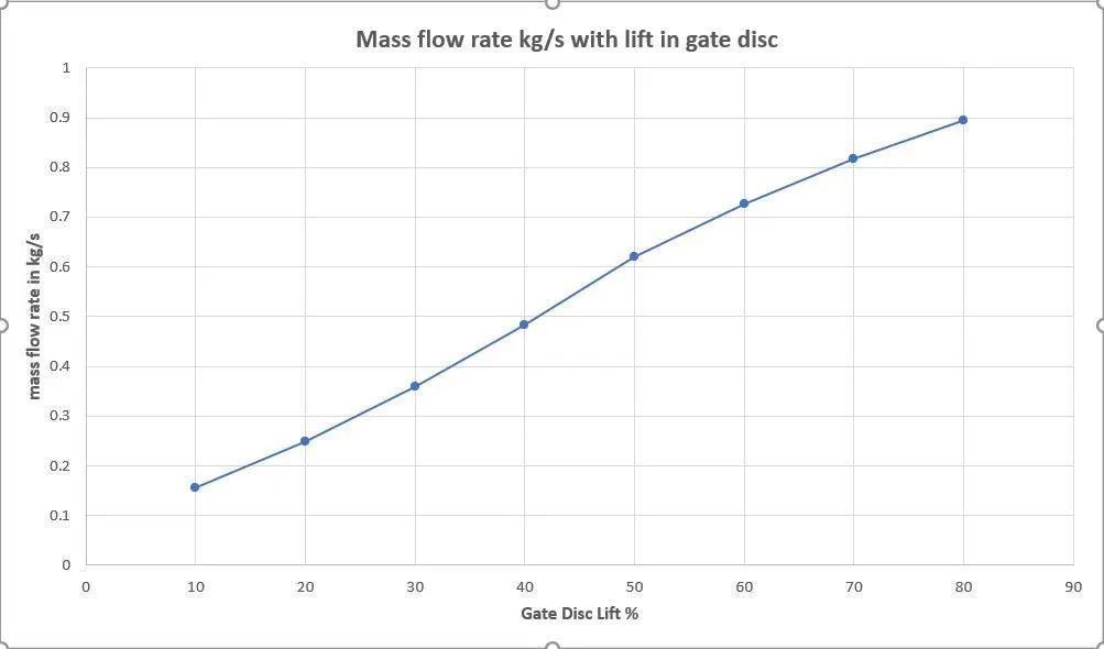
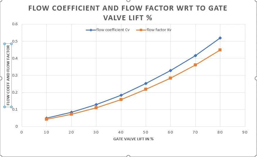
- Calculate the flow coefficient and flow factor for each opening and plot the graph.
- Discuss the results of the mass flow rate and flow coefficient.
Introduction:
In this challenge the gate valve is simulated with flow of water at different lift values ranging from 10% to 80% . The typical total lift is 113.5mm but for the challenge we take in percentage of total. The point of interest in simulating is to get the value of mass flow rate at each lift point and to calculate flow coefficient and flow factor for each point and make a comparitive plot.
Theory:
Gate Valve:
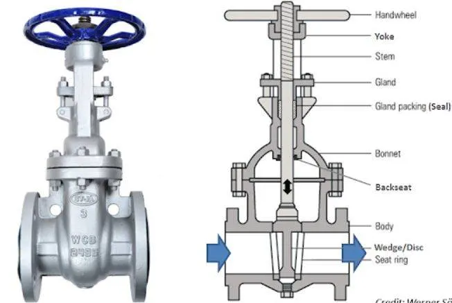
A gate valve, also known as a sluice valve, is a valve that opens by lifting a barrier or gate out of the path of the fluid. Gate valves require very little space along the pipe axis and hardly restrict the flow of fluid when the gate is fully opened. The gate faces can be parallel but are most commonly wedge-shaped.Gate valves are used to shut off the flow of liquids rather than for flow regulation. When fully open, the typical gate valve has no obstruction in the flow path, resulting in very low flow resistance. The size of the open flow path generally varies in a nonlinear manner as the gate is moved. This means that the flow rate does not change evenly with stem travel. Depending on the construction, a partially open gate can vibrate from the fluid flow.
Flow coefficient:
The flow coefficient of a device is a relative measure of its efficiency at allowing fluid flow. It describes the relationship between the pressure drop across an orifice valve or other assembly and the corresponding flow rate.
Mathematically `Cv=Qsqrt((SG)/(DeltaP))`
Q=rate of flow kg/s
SG = specific gravity of fluid(for water 1)
`DeltaP=`pressure drop across the gate valve
Flow factor:
The metric equiavalent of flow factor `Kv`
`Kv=0.865*Cv`
Parametric study:
Parametric study is a good way of calculating multiple outcomes in one go. This really helps to mathematically study variables without going through the hassle of setting up simulation each and every time.
Geometry parameter can be varied in a parametric study without changing the geometry in spaceclaim but simply parametrizing the moving component.
Modelling approach :
- Import the geometry in space claim and lift the valve by 10% and paramtrize the valve.
- Extract the volume with the lift on and supress the physics for remaining all components.
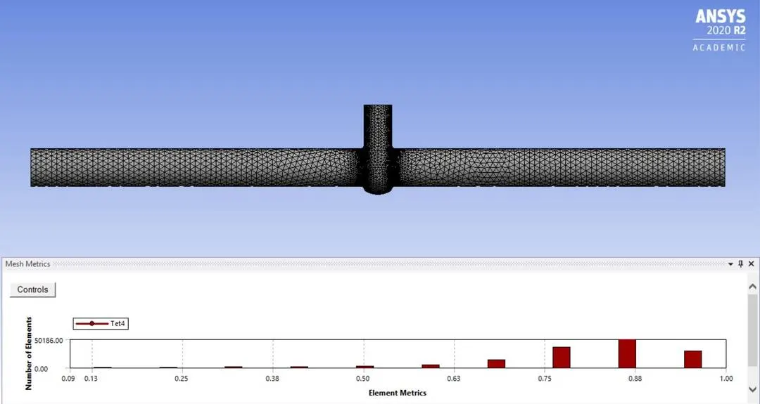
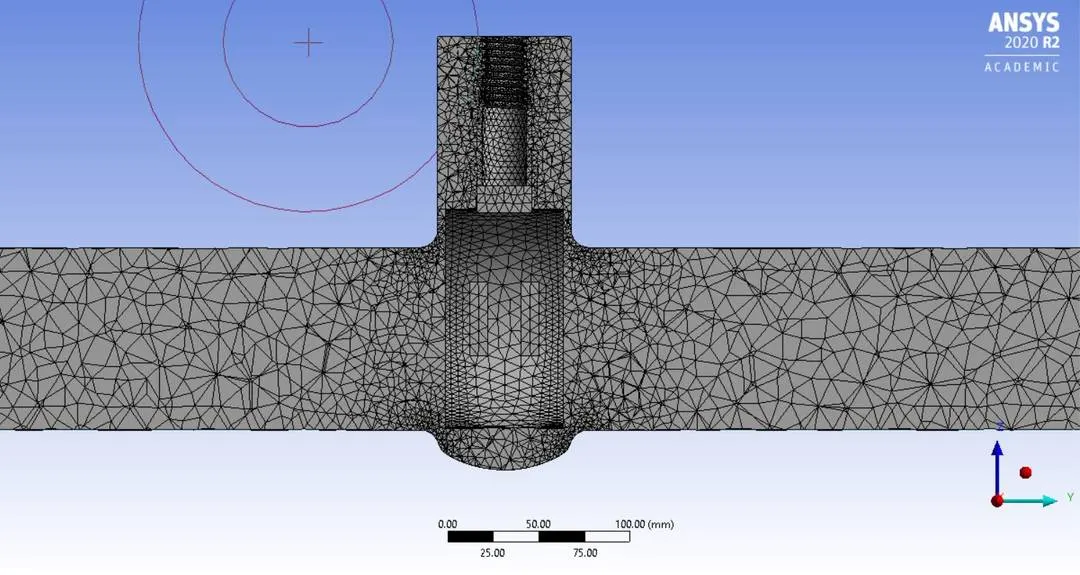
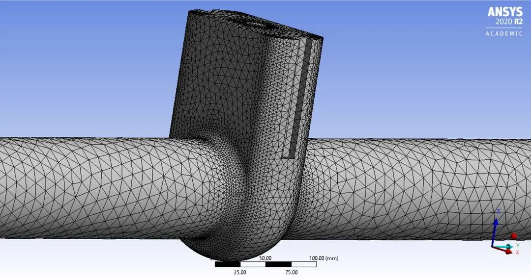
- Mesh the model and assign named selcections.
- open fleunt and set up a steady state simualtion with k -epsilon,realizable ,scalable wall function.
- Boundary condition is pressure inlet and oultet with inlet pressure at 10 pascals.
- check for the mass flow rate at the outlet and pressure drop.
- post process the results for velocity and pressure contours.
Geometry:
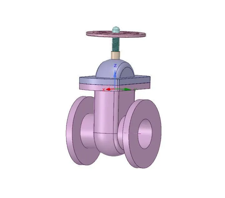
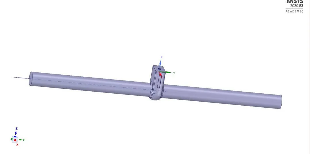
The model is loaded into spaceclaim.
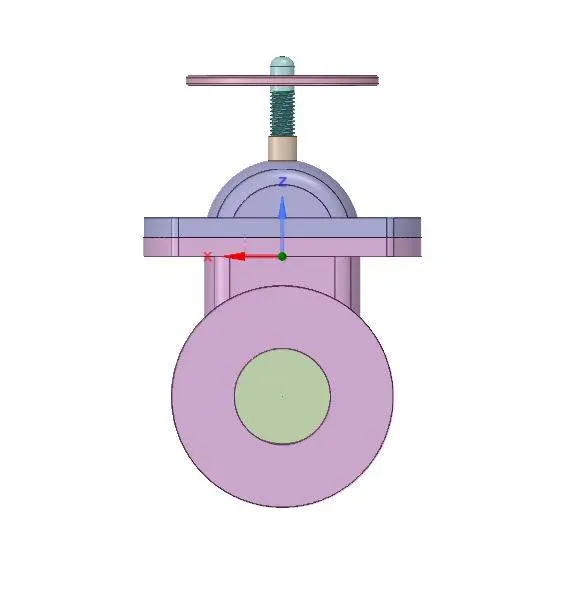
Parametrize the part by moving the gate valve.
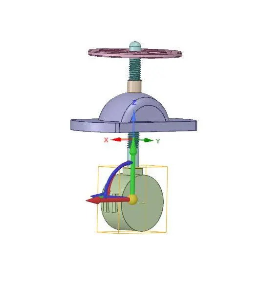
Extracted volume:
Mesh:
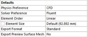

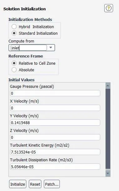
Common fluent setup :
- k-epsilon/Realizable/Scalable wall functions
- water as fluid
- Inlet pressure 10 pascals
- standard initialization
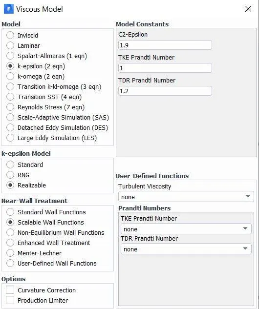
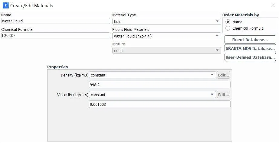
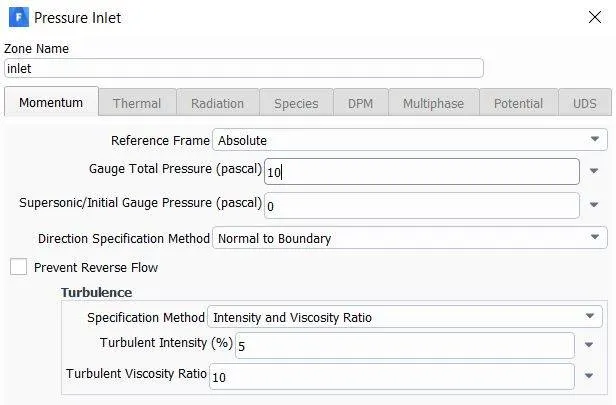
Results:
Parametric solution
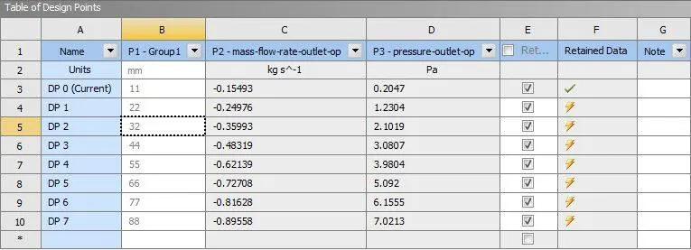
Design point table:
Flow coefficient and Flow factor Calculation :
specific gravity of water - 1000
mass flow rate = taken from table for different lift in kg/s
Pressure inlet= 10 pascals
Presssure outlet = taken from table for different lift in pascals
1.Flow coefficient and flow factor for 10% lift:
Q= 0.15493 kg/s
`Cv=Qsqrt((SG)/(DeltaP))`
=`0.15493sqrt((1)/(10-0.2047))`
Cv= 0.0495
Kv= 0.865*Cv
= 0.865* 0.0495
= 0.0428
Kv= 0.0428
2.Flow coefficient and flow factor for 20% lift:
Q= 0.24976 kg/s
`Cv=Qsqrt((SG)/(DeltaP))`
=`0.24976sqrt((1)/(10-1.2304))`
Cv= 0.0843
Kv= 0.865*Cv
= 0.865* 0.0843
= 0.0729
Kv= 0.0729
3.Flow coefficient and flow factor for 30% lift:
Q= 0.35993 kg/s
`Cv=Qsqrt((SG)/(DeltaP))`
=`0.35993sqrt((1)/(10-2.1019))`
Cv= 0.1280
Kv= 0.865*Cv
= 0.865* 0.1280
= 0.1107
Kv= 0.1107
4.Flow coefficient and flow factor for 40% lift:
Q= 0.48319 kg/s
`Cv=Qsqrt((SG)/(DeltaP))`
=`0.48319sqrt((1)/(10-3.0807))`
Cv= 0.1837
Kv= 0.865*Cv
= 0.865* 0.1837
= 0.1589
Kv= 0.1589
5.Flow coefficient and flow factor for 50% lift:
Q= 0.62139 kg/s
`Cv=Qsqrt((SG)/(DeltaP))`
=`0.62139sqrt((1)/(10-3.9804))`
Cv= 0.2533
Kv= 0.865*Cv
= 0.865* 0.2533
= 0.2191
Kv= 0.2191
6.Flow coefficient and flow factor for 60% lift:
Q= 0.72708 kg/s
`Cv=Qsqrt((SG)/(DeltaP))`
=`0.72708sqrt((1)/(10-5.092))`
Cv= 0.3281
Kv= 0.865*Cv
= 0.865* 0.3281
= 0.2839
Kv= 0.2839
7.Flow coefficient and flow factor for 70% lift:
Q= 0.81628 kg/s
`Cv=Qsqrt((SG)/(DeltaP))`
=`0.81628sqrt((1)/(10-6.1555))`
Cv= 0.4163
Kv= 0.865*Cv
= 0.865* 0.4163
= 0.3601
Kv= 0.3601
8.Flow coefficient and flow factor for 80% lift:
Q= 0.89558 kg/s
`Cv=Qsqrt((SG)/(DeltaP))`
=`0.89558sqrt((1)/(10-7.0213))`
Cv= 0.5189
Kv= 0.865*Cv
= 0.865* 0.5189
= 0.4488
Kv= 0.4488
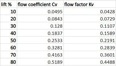
Lift table:
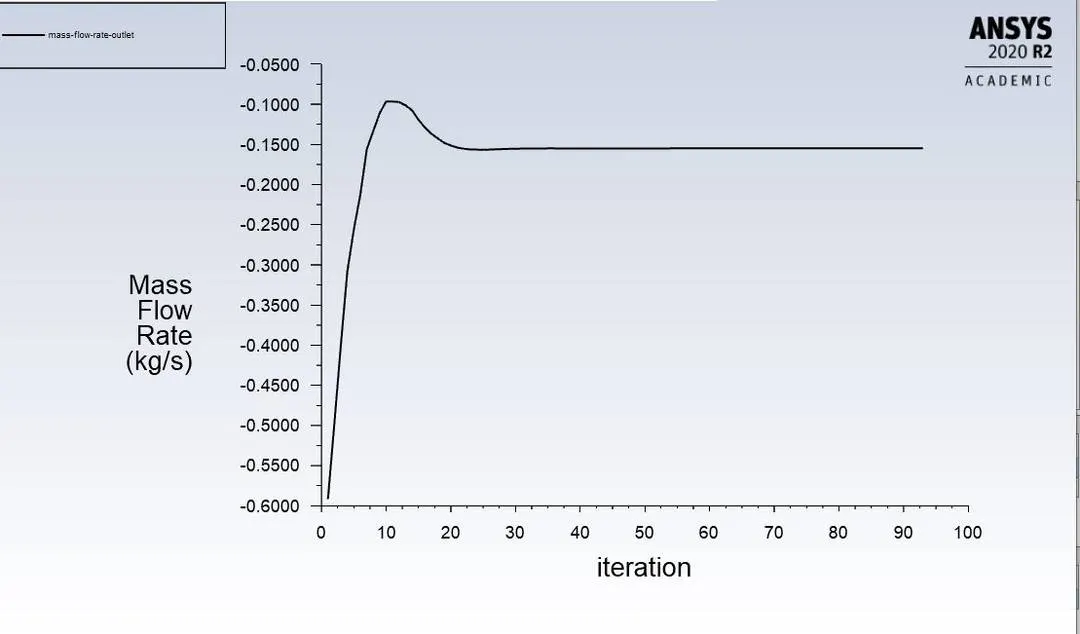
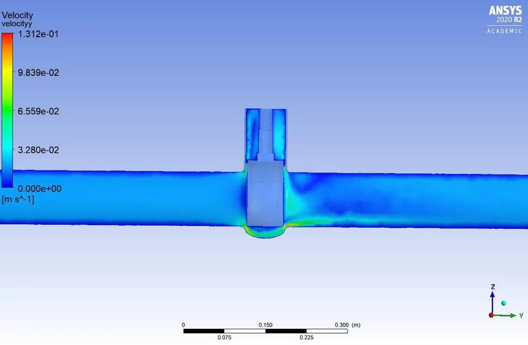
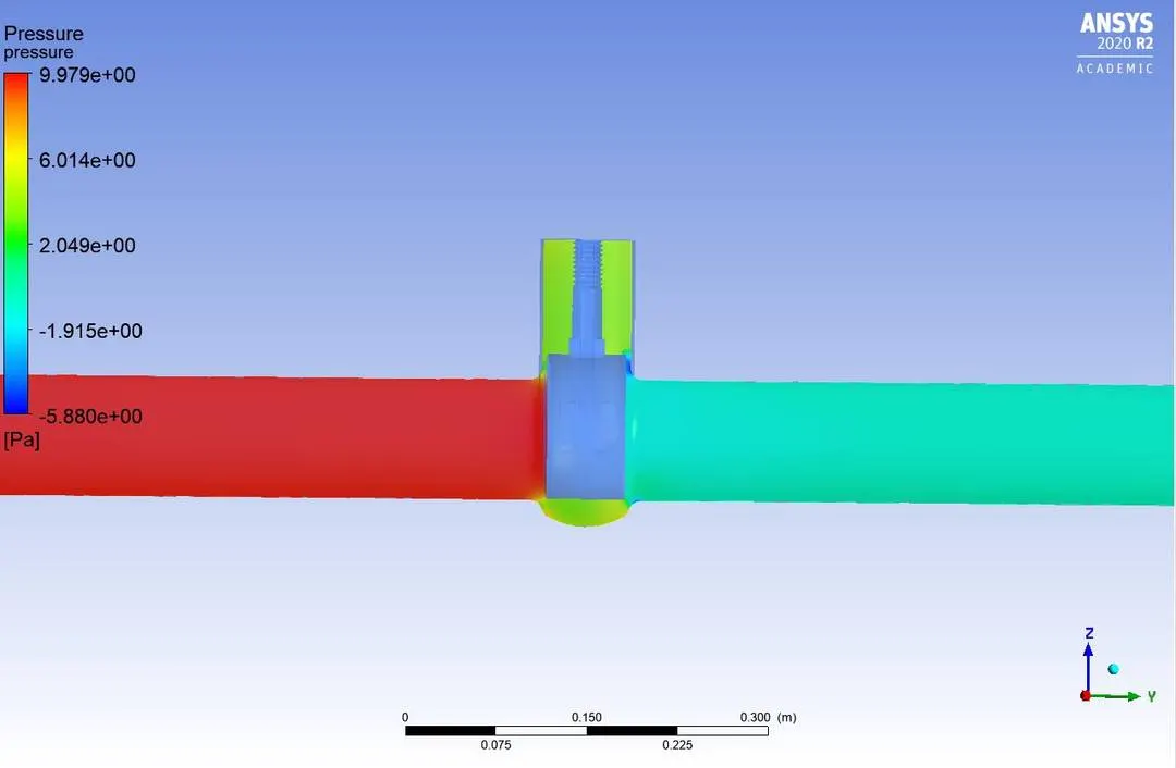
Results for lift of 10%:
Mass flow rate:
Velocity contour:
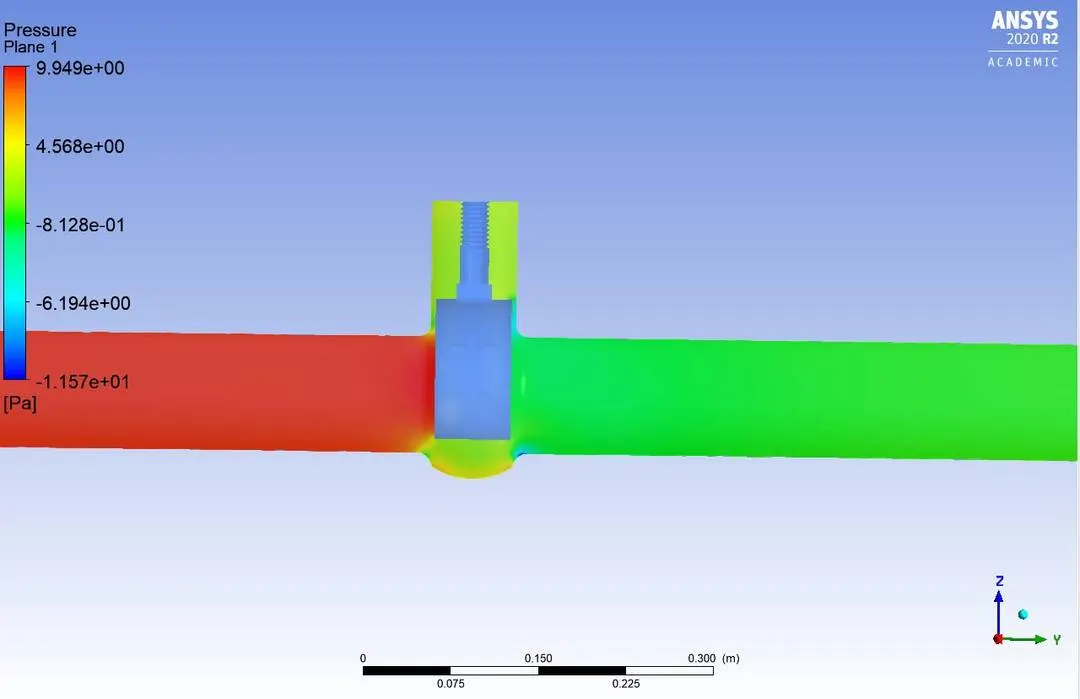
Pressure contour:
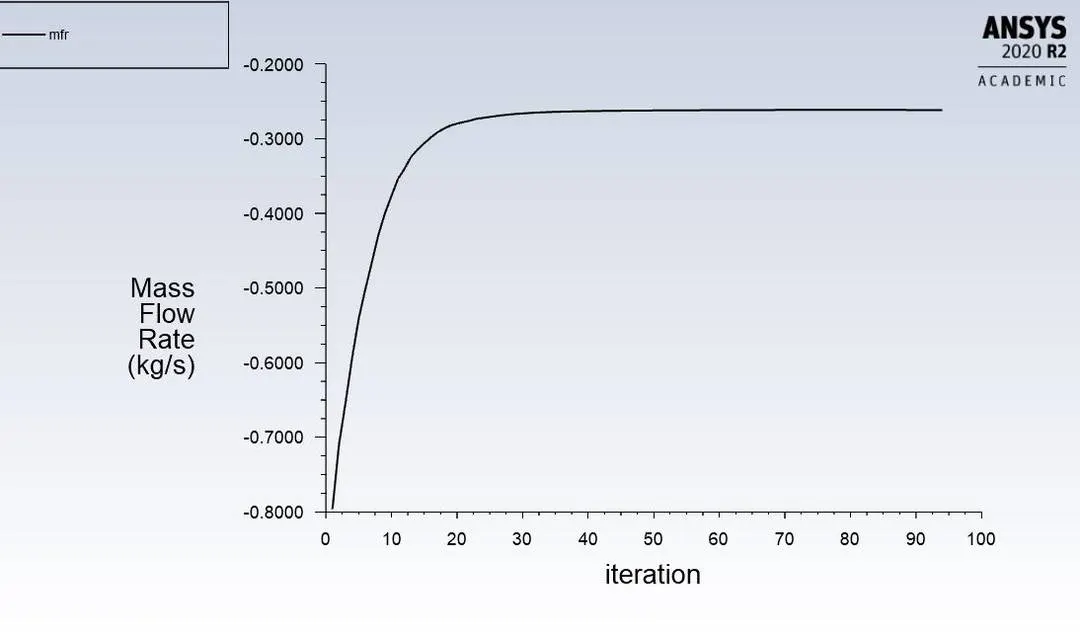
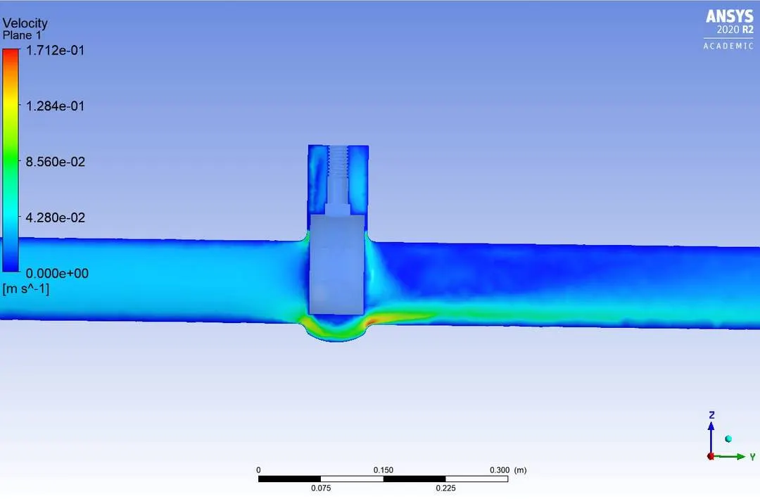
Results for lift of 20%:
Mass flow rate:
Velocity contour:
Pressure contour:
Results for lift of 30%:
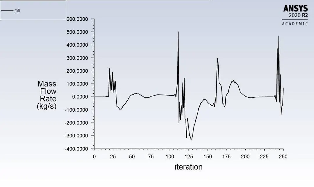
Mass flow rate:
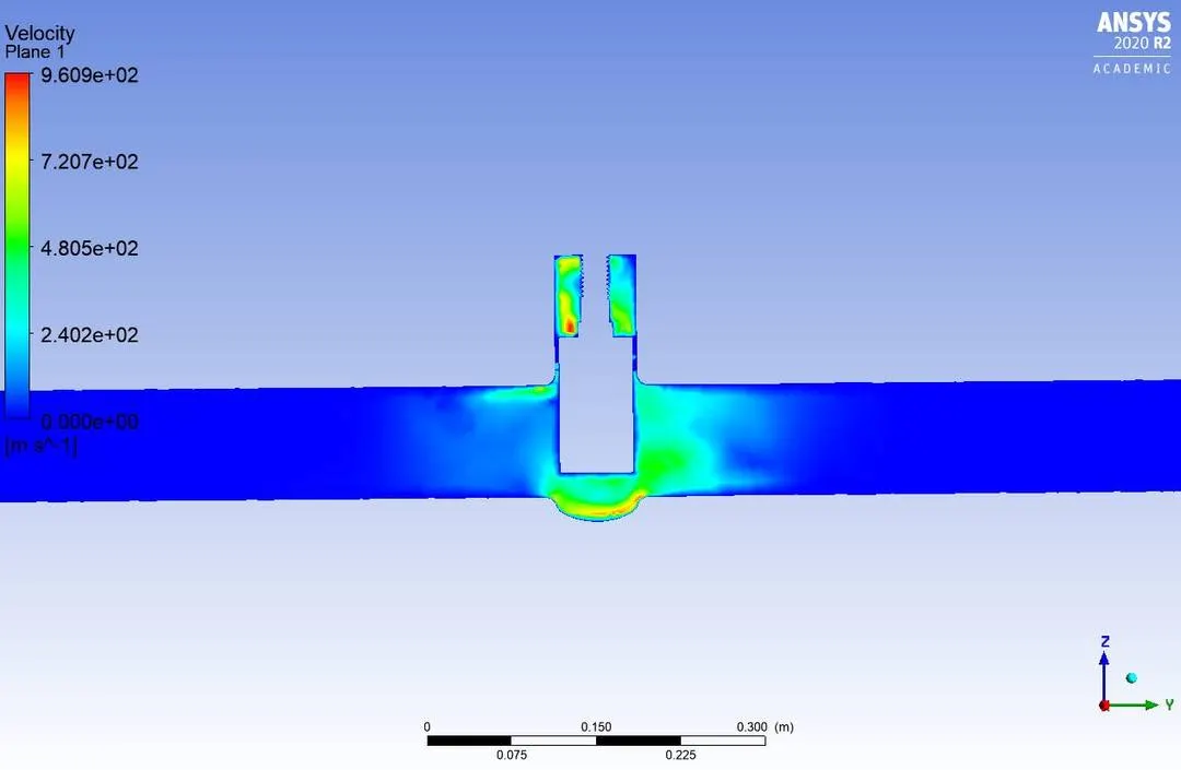
Velocity contour:
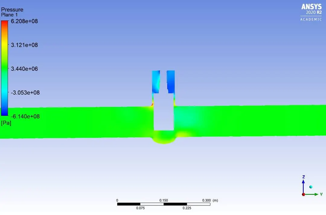
Pressure contour:
Results for lift of 40%:
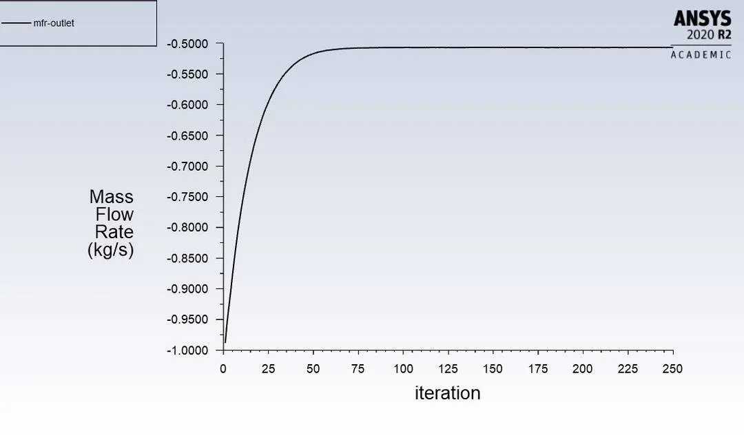
Mass flow rate:
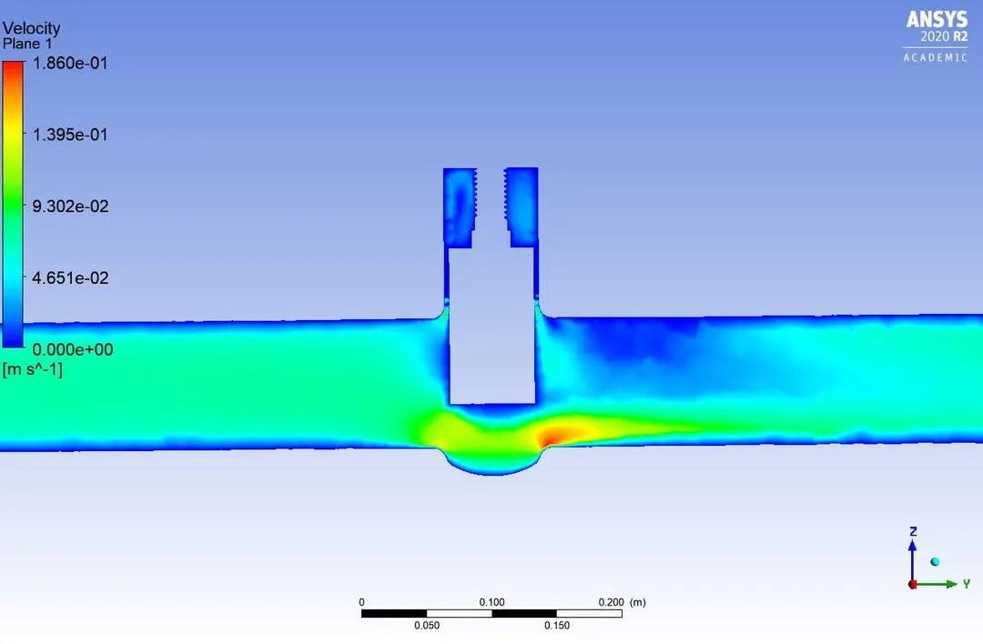
Velocity contour:
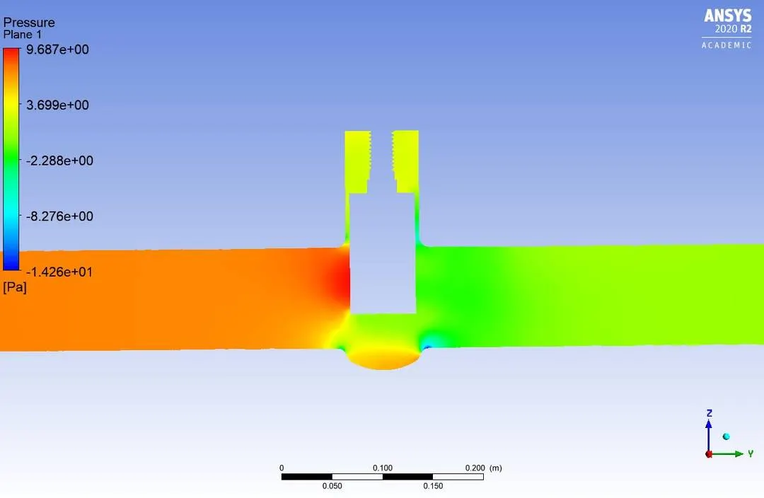
Pressure contour:
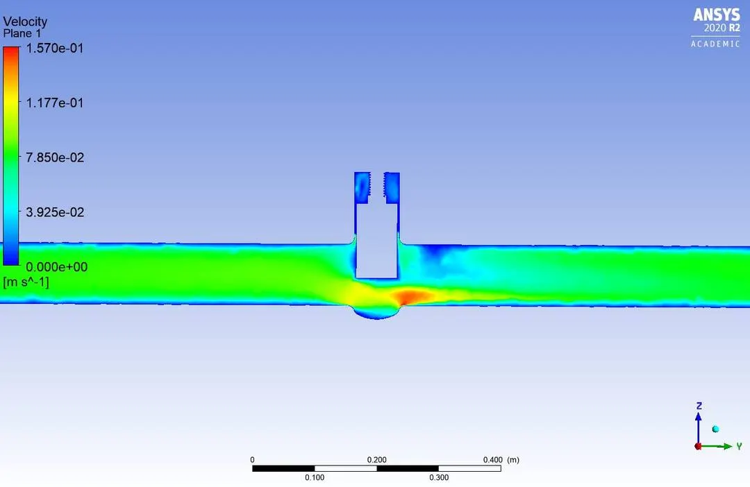
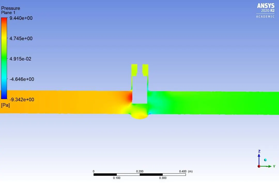
Results for lift of 50%:
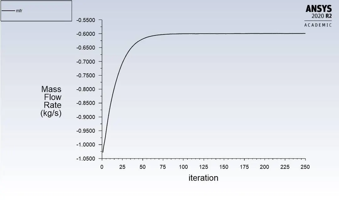
Mass flow rate:
Velocity contour:
Pressure contour:
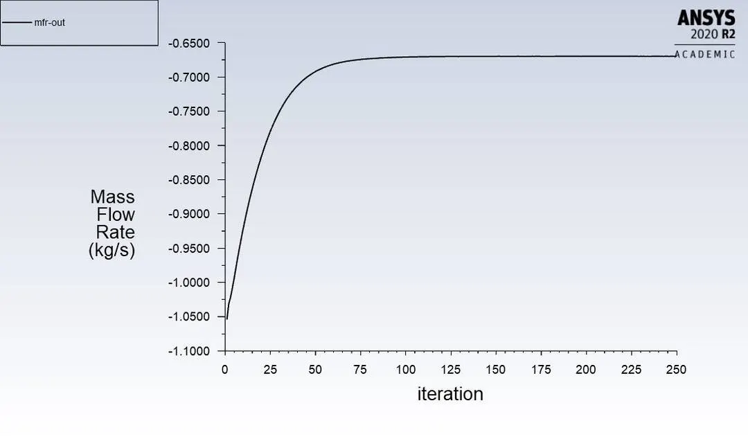
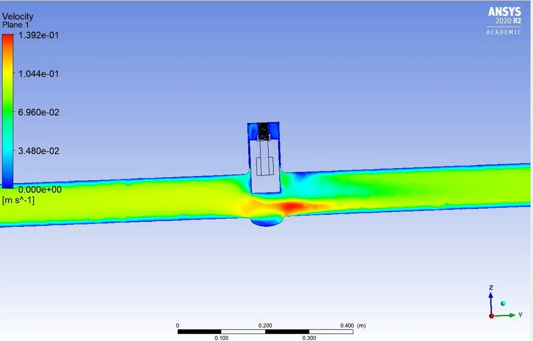
Results for lift of 60%:
Mass flow rate:
Velocity contour:
Pressure contour:
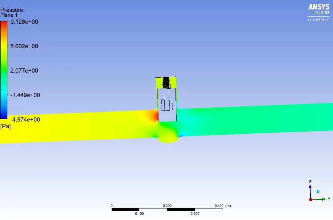
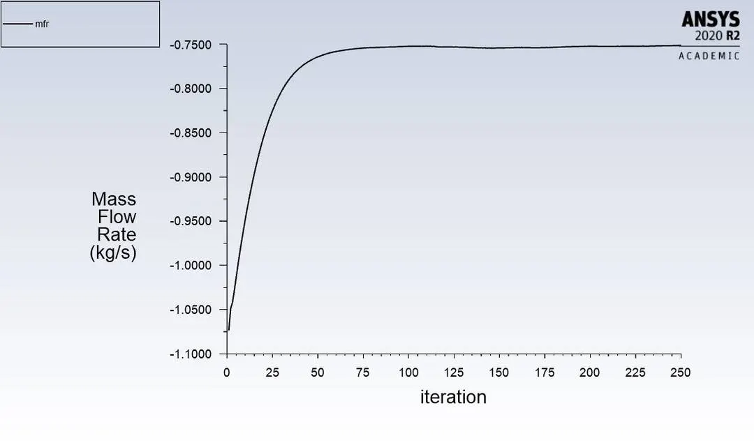
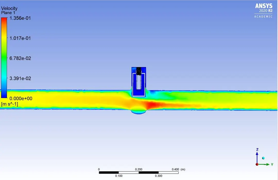
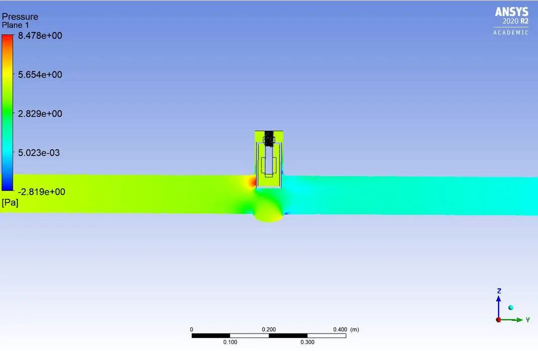
Results for lift of 70%:
Mass flow rate:
Velocity contour:
Pressure contour:
Results for lift of 80%:
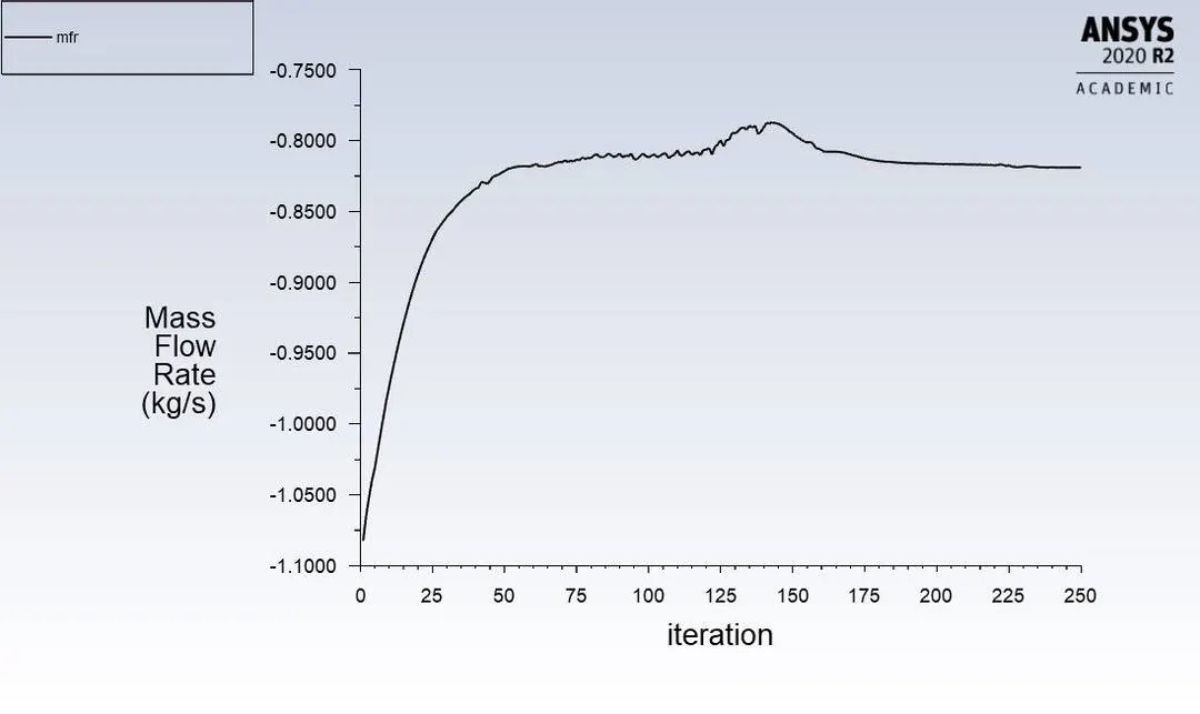
Mass flow rate:
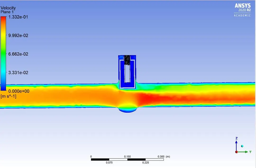
Velocity contour:
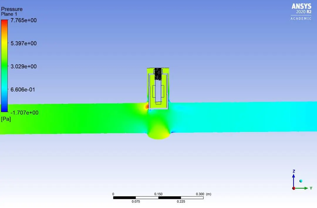
Pressure contour:
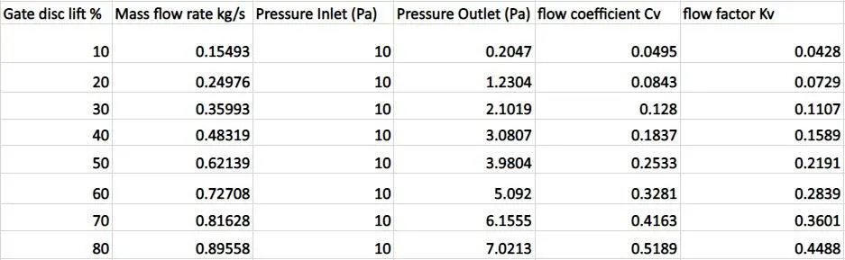
Final Result table:
Final chart plots:
Mass flow rate in kg/s vs gate disc lift (%)
Flow coefficient and flow factor wrt to gate disc lift %
Results and inferences:
- The mass flow rate with each value of lift increases which tells that the simulationis correct.
- The flow factor have lesser values than the flow coefficient.
- For each value of lift we can see a positive increment in lift.
- For each value of increasing lift pressure at outlet increases which directly indicates increased flow area.
- Parametric study gives a better and speedy results without going through a hassle of setting up simulation each and every time.