Week 3 - Taylor table method and Matlab code

Three numerical approximation for the function `f(x)=e^xcos(x)`.

In this we basically solve for fourth order approximation for 2nd order derivative of the above function

second derivative: `f''(x)=-2*e^xsin(x)`

we solve for central differencing,skewed right and skewed left sided difference

matrices A1,A2,A3 :

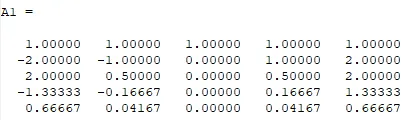
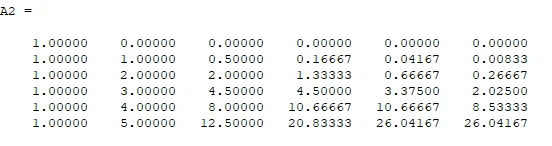
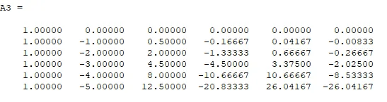
three OUTPUT coefficient matrices(x1,x2,x3):

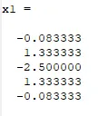
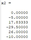
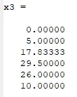
x1 has five coefficients a1,b1,c1,d1,e1

x2 has six coefficients a2,b2,c2,d2,e2,g2

x3 has six coefficients a3,b3,c3,d3,e3,g3

analytical second derivative of function: -4.5747

Code for the approximation and error :

clear all
close all
clc

% second order derivative of f(x)=e^(x)*cos(x)
x=linspace(pi/3,pi/6,5)
dx=linspace(pi/4,pi/400,20);
  for i=1:5

for j=1:x
analytical_derivative(i) = -2*e^(j)*sin(j)
end

%central diff
A1=[1 1 1 1 1;-2 -1 0 1 2;2 1/2 0 1/2 2;-8/6 -1/6 0 1/6 8/6;16/24 1/24 0 1/24 16/24]
%X1=[a1;b1;c1;d1;e1];
B1=[0;0;1;0;0]
x1=inv(A1)*B1;
a1=x1(1);
b1=x1(2);
c1=x1(3);
d1=b1;
e1=a1;
central_diff=((2*a1)+(b1/2)+(d1/2)+(2*e1));
error1(i)=abs(central_diff-analytical_derivative(i))

%skewed right
A2=[1 0 0 0 0 0;1 1 1/2 1/6 1/24 1/120;1 2 4/2 8/6 16/24 32/120;1 3 9/2 27/6 81/24 243/120;1 4 16/2 64/6 256/24 1024/120;1 5 25/2 125/6 625/24 3125/120]
B2=[0;0;1;0;0;0];
x2=inv(A2)*B2;
a2=x2(1);
b2=x2(2);
c2=x2(3);
d2=x2(4);
e2=x2(5);
g2=x2(6);
skewed_right=((b2/2)+((4*c2)/2)+((9*d2)/2)+((16*e2)/2)+((25*g2)/2));
error2(i)=abs(skewed_right-analytical_derivative(i))


A3=[1 0 0 0 0 0;1 -1 1/2 -1/6 1/24 -1/120;1 -2 4/2 -8/6 16/24 -32/120;1 -3 9/2 -27/6 81/24 -243/120;1 -4 16/2 -64/6 256/24 -1024/120;1 -5 25/2 -125/6 625/24 -3125/120]
B3=[0;0;1;0;0;0];
x3=inv(A3)*B3;
a3=x3(1);
b3=x3(2);
c3=x3(3);
d3=x3(4);
e3=x3(5);
g3=x3(6);
skewed_left=((b3/2)+((4*c3)/2)+((9*d3)/2)+((16*e3)/2)+((25*g3)/2));
error3(i)=abs(skewed_left-analytical_derivative(i))
end




figure(1)
loglog(dx,error1(i),'*')
hold on
loglog(dx,error2(i),'o')
hold on
loglog(dx,error3(i),'^')
legend('-*-central_diff','-o-skewed_right','-^-skewed_left')
xlabel('dx')
ylabel('error')

outputs:

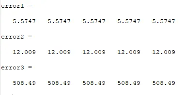
PLOT

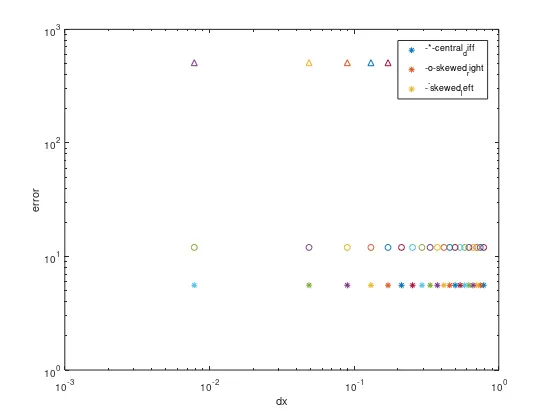
* central difference

o skewed right sided difference

^ skewed left sided difference

explanation for code:

• In the code the basic 2nd derivative of function is computed analytically.
• three outputs are needed so i made matrices A1,A2,A3 and listed out B1,B2,B3 and calculated the inverse
• after getting the inverse the formula of three approximations i.e central,skewed right,skewed left are computed
• now error is computed
• now log plot is generated between dx and three errors

explanation for plot:

• the log plot is generated to get a better viewing perspective
• as we can see the central diffrerncing comes out to be the least error term
• central differnce<skewed right<skewed left
• according to the computation central difference gives the least error as more terms are not computed to extremes(extreme right and left) of the numerical stencil.
• by this computation more the skeweness or skewed difference terms are involved more is the error obtained.
• so CD can really neutralize or display a logical error based plot with least error where both skewed right and left cannot.