Conjugate Heat Transfer Analysis on a graphics card.

Aim: To perform Conjugate heat transfer analysis on a graphics card:

Introduction:

In this project we will simulate conjagate heat transfer on graphic card. Graphics card is an essential component in computer and laptop so keeping it cool or at optimum temperature is needed for overall computer performance. It mainly has three components which are Pcb, processor and fins.Cooling of graphic card is done by forced convection by flowing air by fans on to the fins of the graphic card. The power heating of graphic card depends on the power consumption of the processor . Higher the power consumption higher is the heat generated so we need faster cooling to make sure the processor is at its optimum temperature or else the processor may fail to run and the system shuts down. The crux of this simulation is to see how much of cooling is done while varying the inlet air speed.

Theory:

Conjugate heat transfer analysis:

The term conjugate heat transfer (CHT) is used to describe processes which involve variation of temperature within solids and fluids because of thermal interaction between solids and fluids.The rate of heat transfer is directly proportional to the temperature difference. In solids the conduction dominates and in fluids convection dominates. Efficiently combining both fluids and solids is a key to design any heat involving machine.

Heat transfer in solids and heat transfer in fluids are combined in majority of applications. This is because fluid flow around solids and the fact that solids are immersed in fluid. For example a hot cup of water is surrounded by ambient air. The basic crux of applying CHT analysis is getting understanding for how can we incorporate a solid and fluid interactions with required amount of heat transfer between them.

Modelling Approch:

• Importing model in spaceclaim and making it mesh ready by sharing its topology.
• Assigning named selection to each of the component by selecting them individually.
• One coarse mesh and a refined meshing is done.
• For setting up fluent by using k-epsilon turbulence model for steady state simulation.
• Assign materials to different components.
• Assigning boundary conditions for solid and fluid zones.
• A 30 watt power utilizing processor is taken.
• Run the simulation till the solution has converged.
• Post process the results.

Geometry:

Basic model:

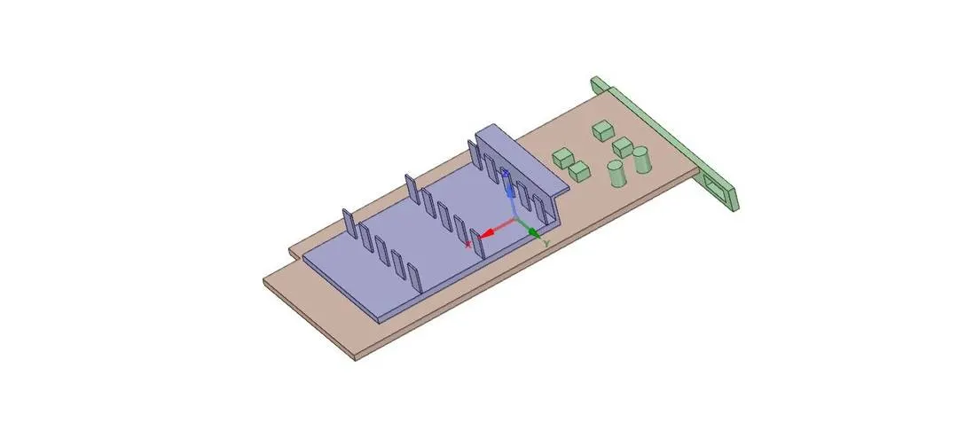
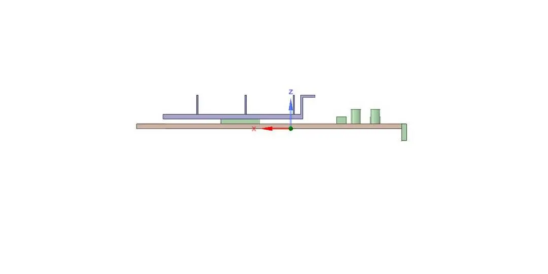
Front view:

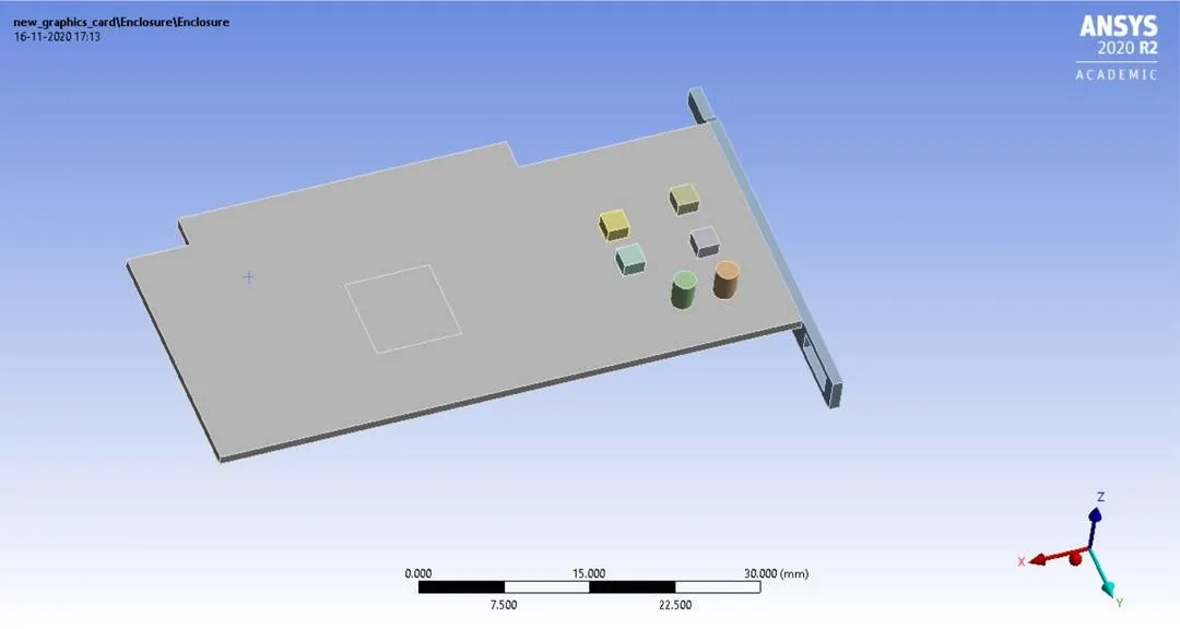
Individual components:

PCB board

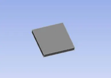
Processor:

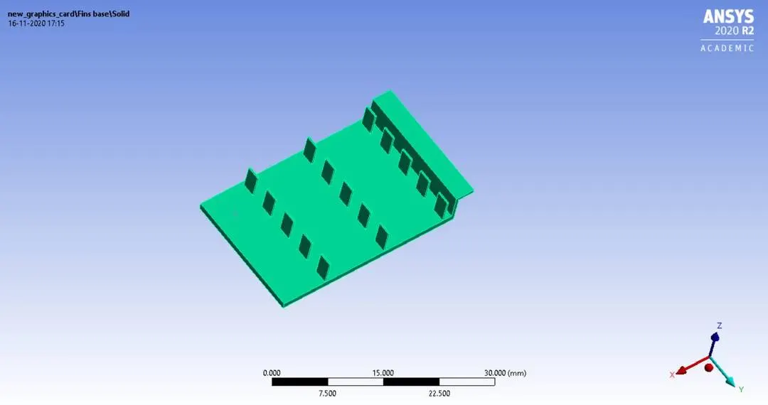
Fins:

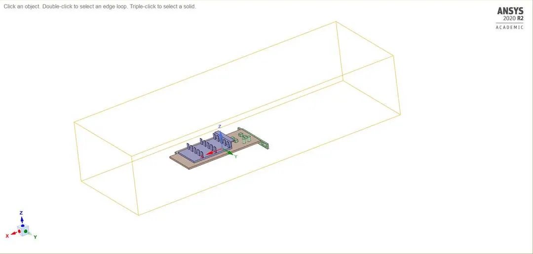
Enclosed volume:

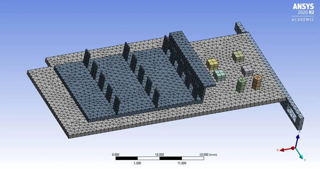
Mesh:

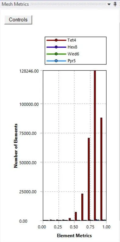
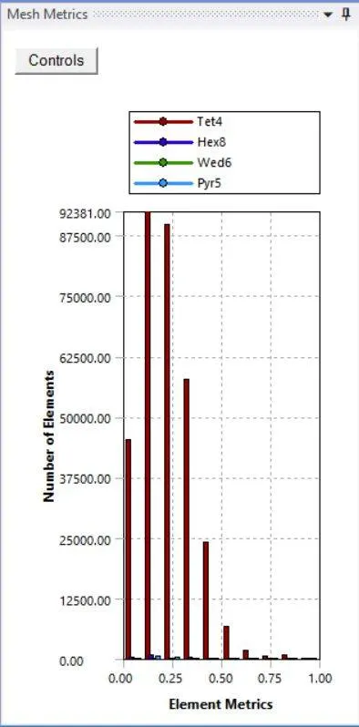
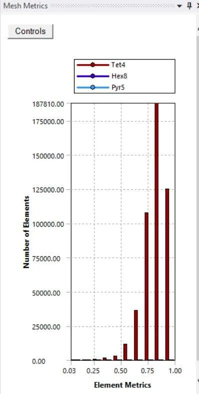
Baseline mesh :

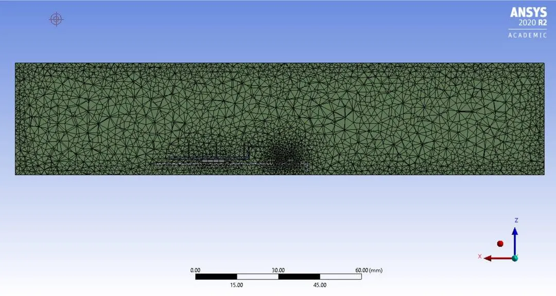
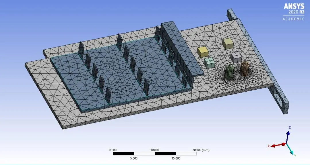
element quality skeweness

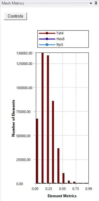
Refined Mesh:

Element quality skewness

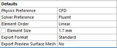
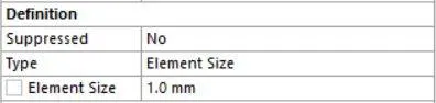
Element size Body sizing

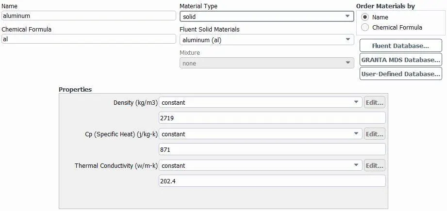
Material properties:

Pcb is of aluminum

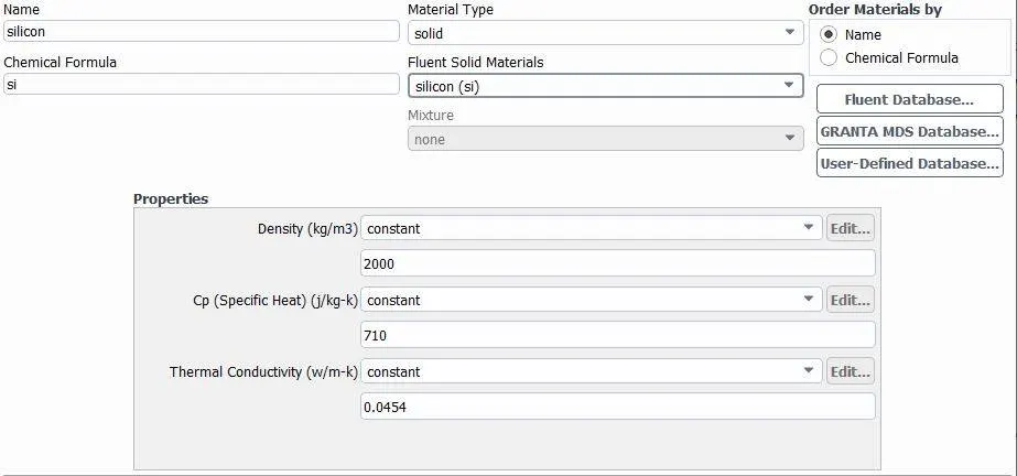
processor is of silicon

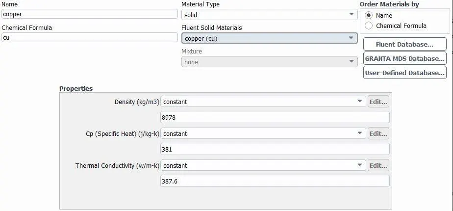
Fins are of copper

Case setup in fluent:

• Solver - pressure based steady state solver
• Energy equation included
• k-epsilon turbulence model

Boundary conditions:

Calculation for Reynolds number:

For Reynolds number calculation we need to find the hydraulic diameter of the enclosure

`Area= 65mm*40.5mm=2632.5mm^2`

`Perimeter=211mm`

Hydraulic diameter : `Dh=(4*A)/(P)=(4*65*40.5*10^-6)/(211*10^-3)=0.05m`

Reynolds number : `(rho*V*Dh)/(mu)=(1.225*1*0.05)/(1.7894*10^-5)=3422`----velocity 1 m/s

Reynolds number : `(rho*V*Dh)/(mu)=(1.225*3*0.05)/(1.7894*10^-5)=10269`---velocity 3 m/s

Reynolds number : `(rho*V*Dh)/(mu)=(1.225*5*0.05)/(1.7894*10^-5)=17115`---velocity 5 m/s

Calculation for heat generated by processor:

The geometry of preocessor has dimensions 8mm*8mm*1mm

The power consumption for the processor is around 30 watts

Heat generated : `(30)/(64*10^-9)=468,750,000 w/m^3` -----source term

Case Table:

Case 1 : Baseline mesh

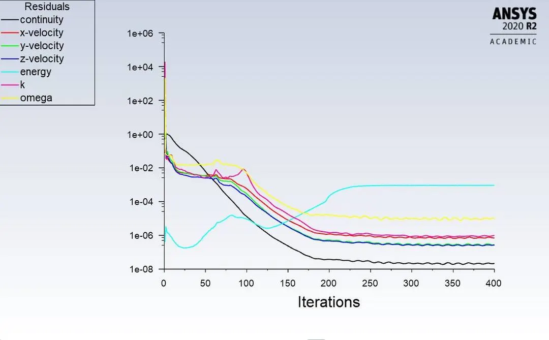
Residuals: soluton is converged

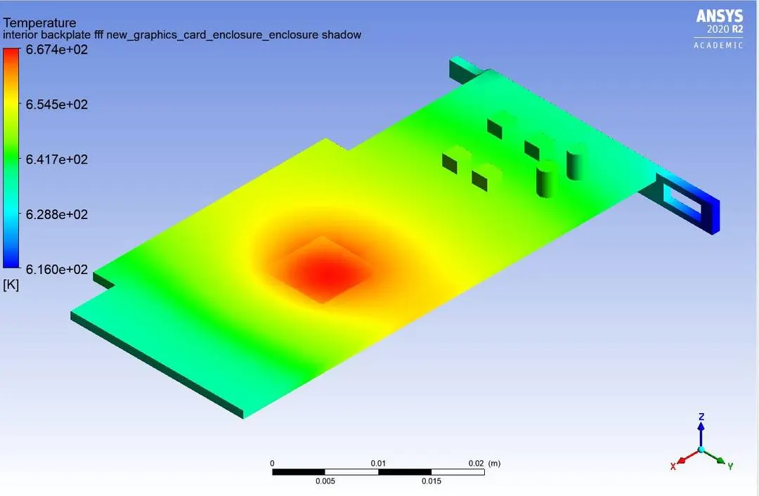
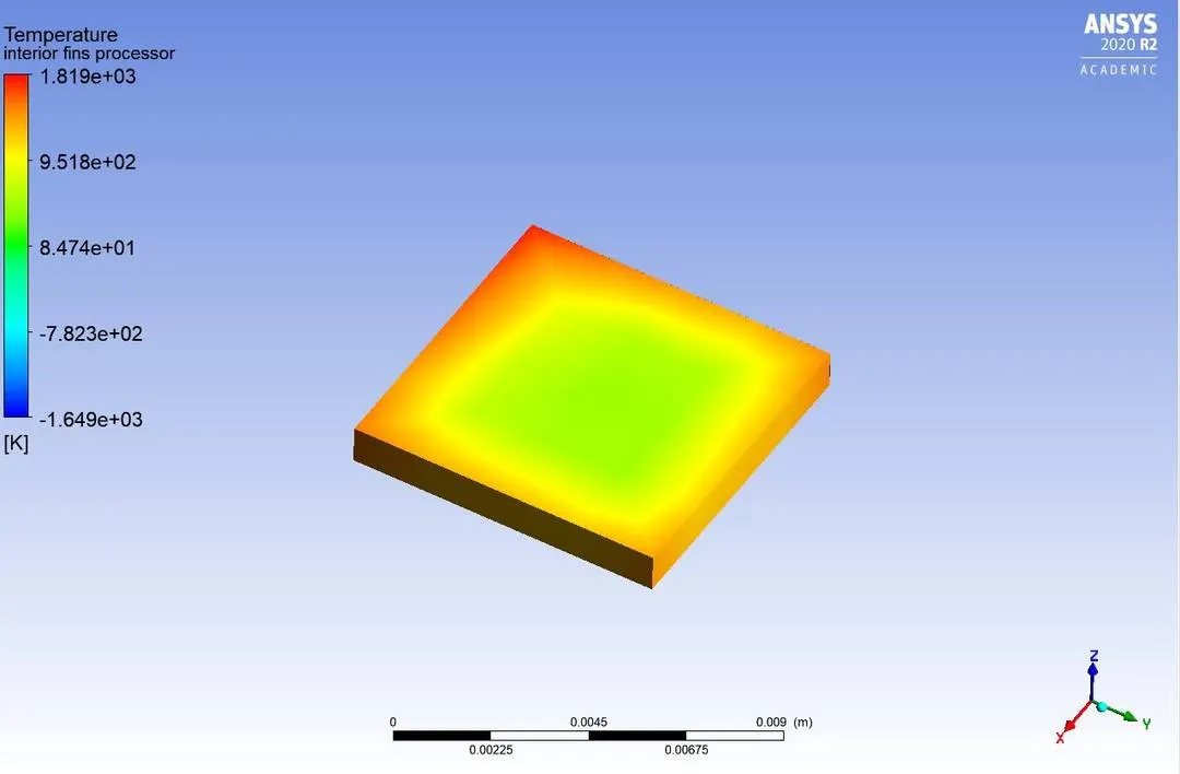
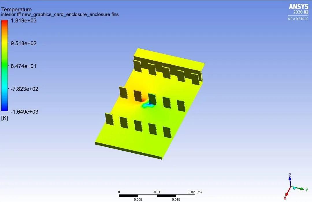
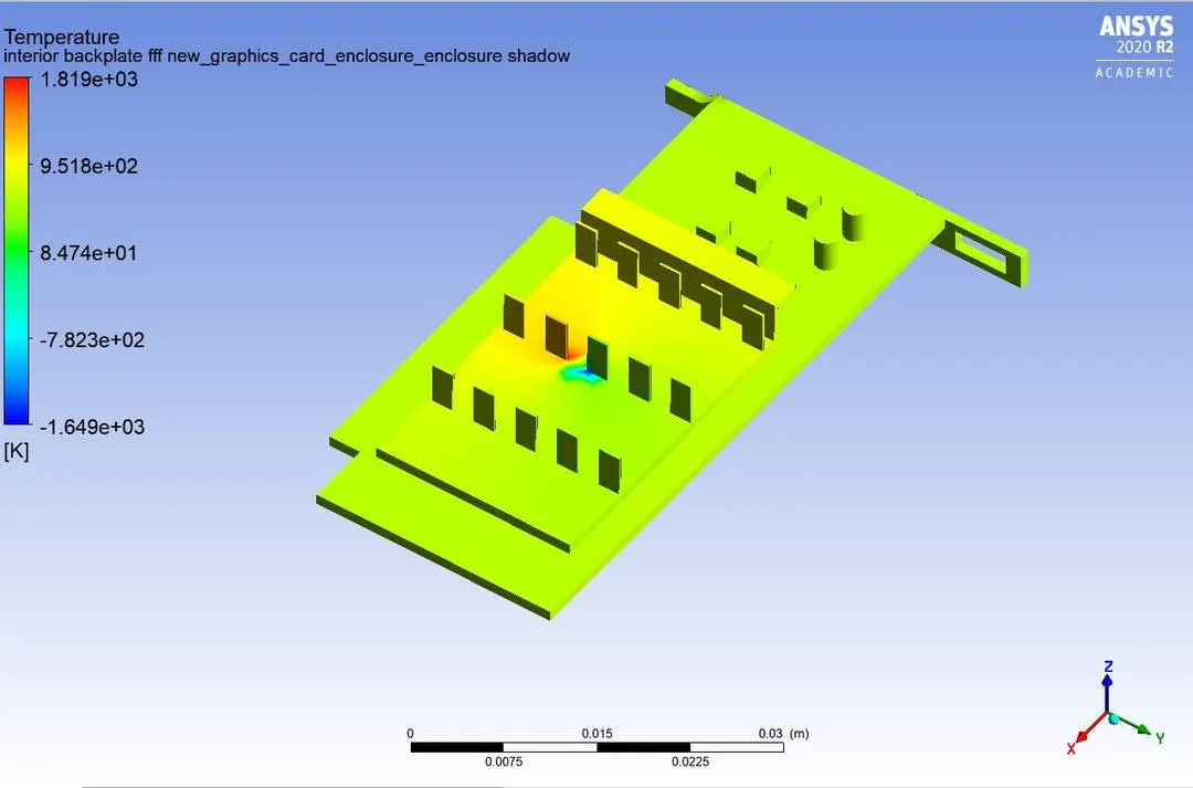
Temperature contour:

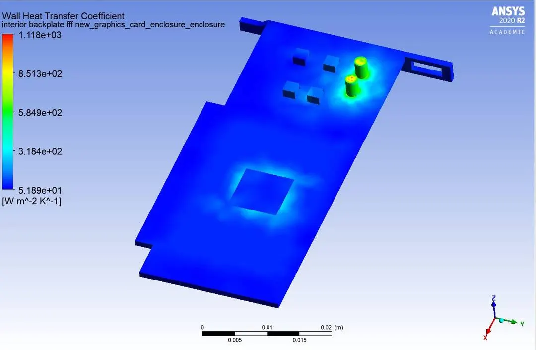
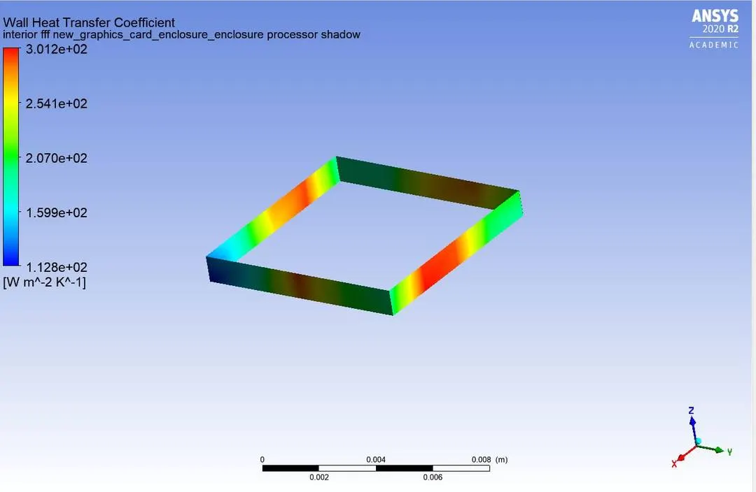
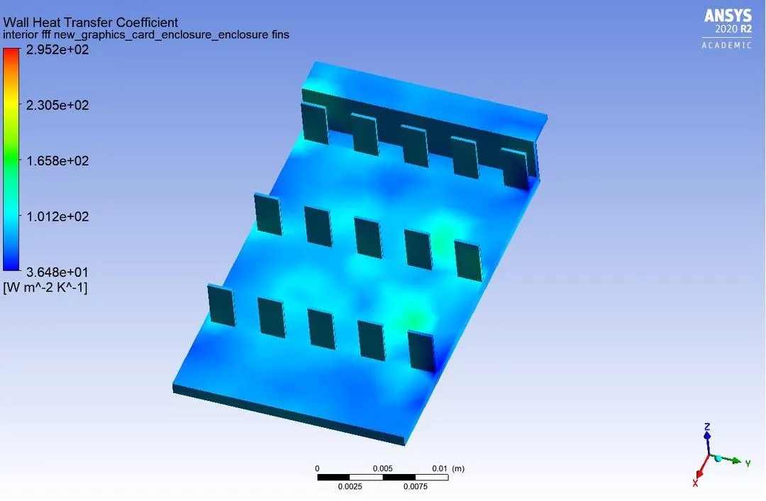
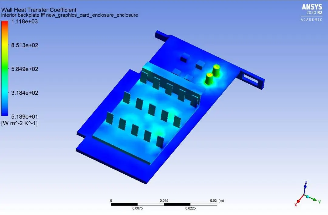
Heat transfer coefficient:

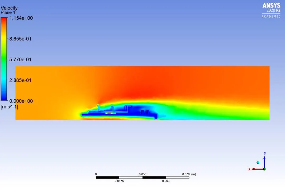
velocity plane:

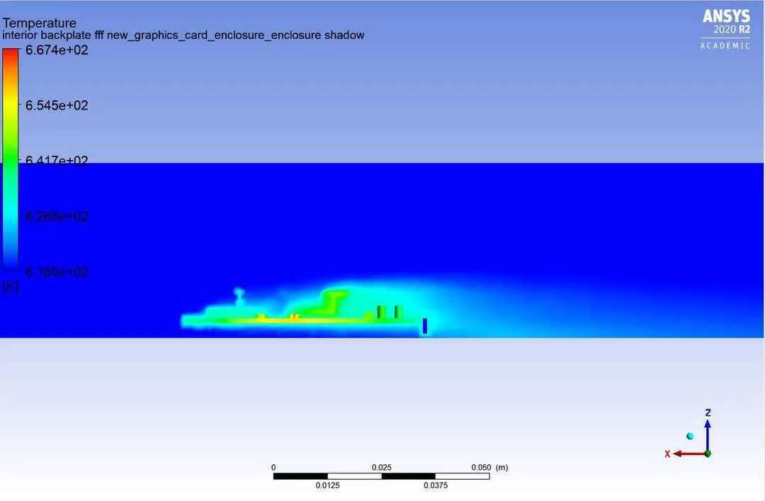
Temperature plane:

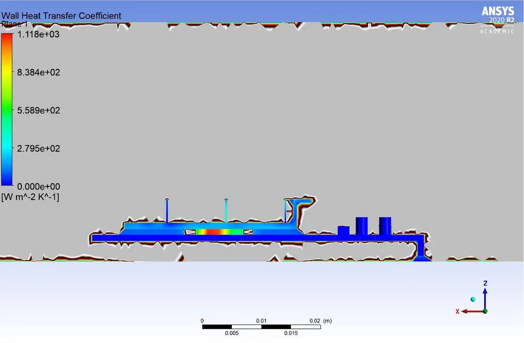
wall heat transfer coefficient plane:

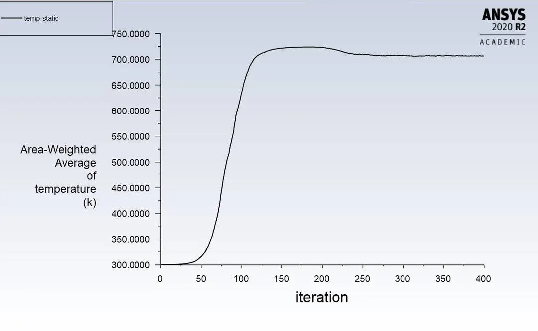
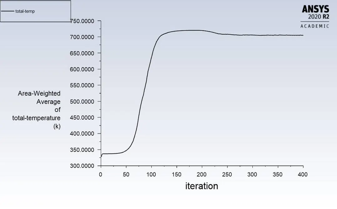
temperature plot:

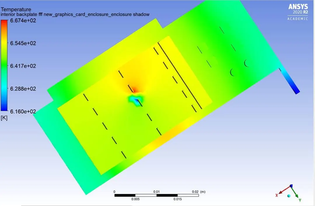
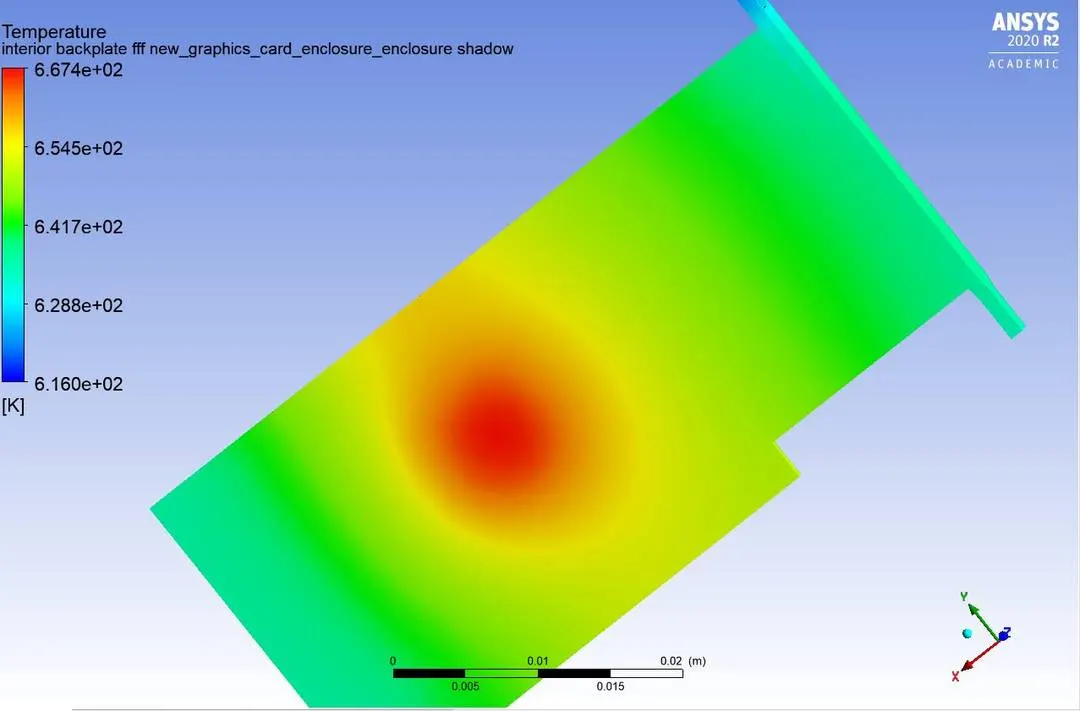
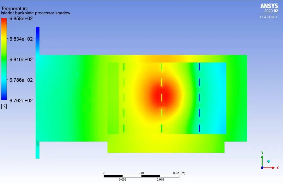
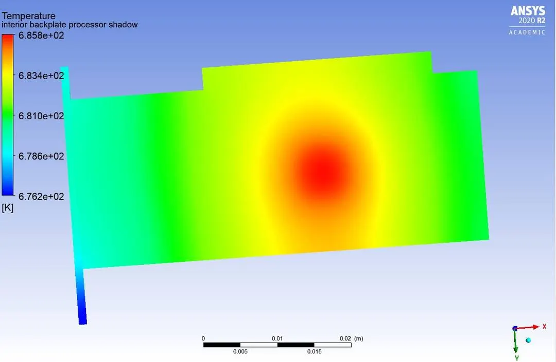
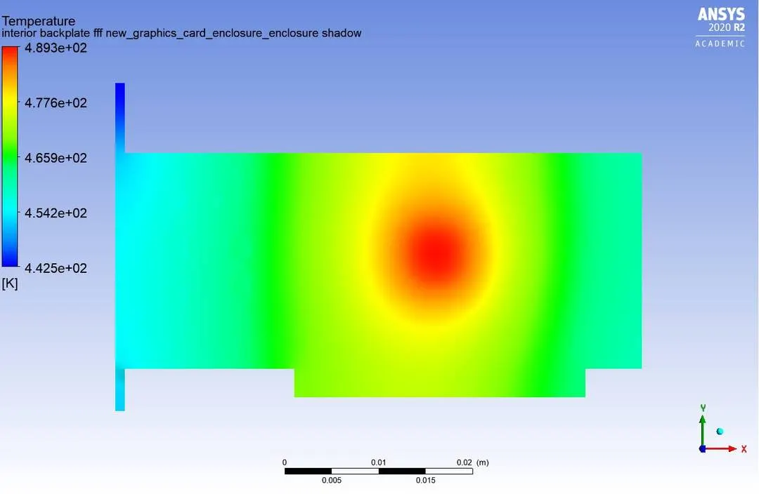
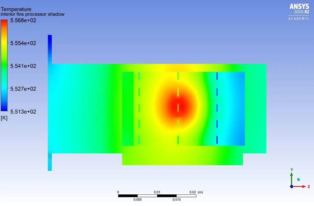
Hotspot areas:

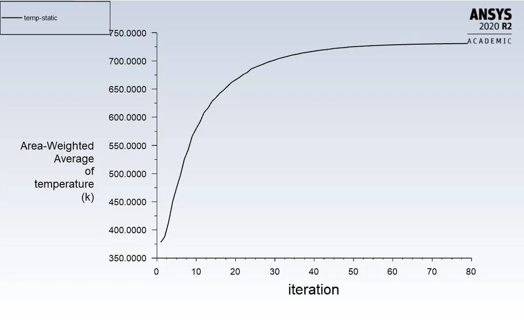
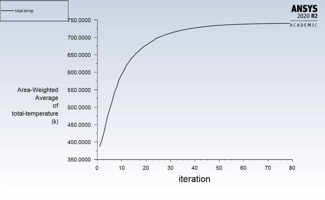
Case 2: Refined mesh v=1 m/s

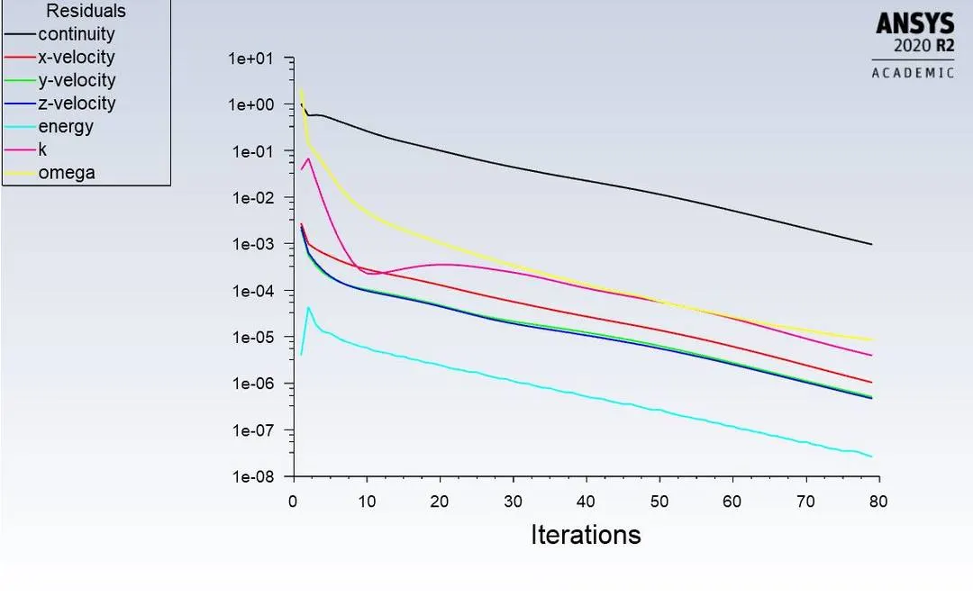
Residuals: soluton is converged

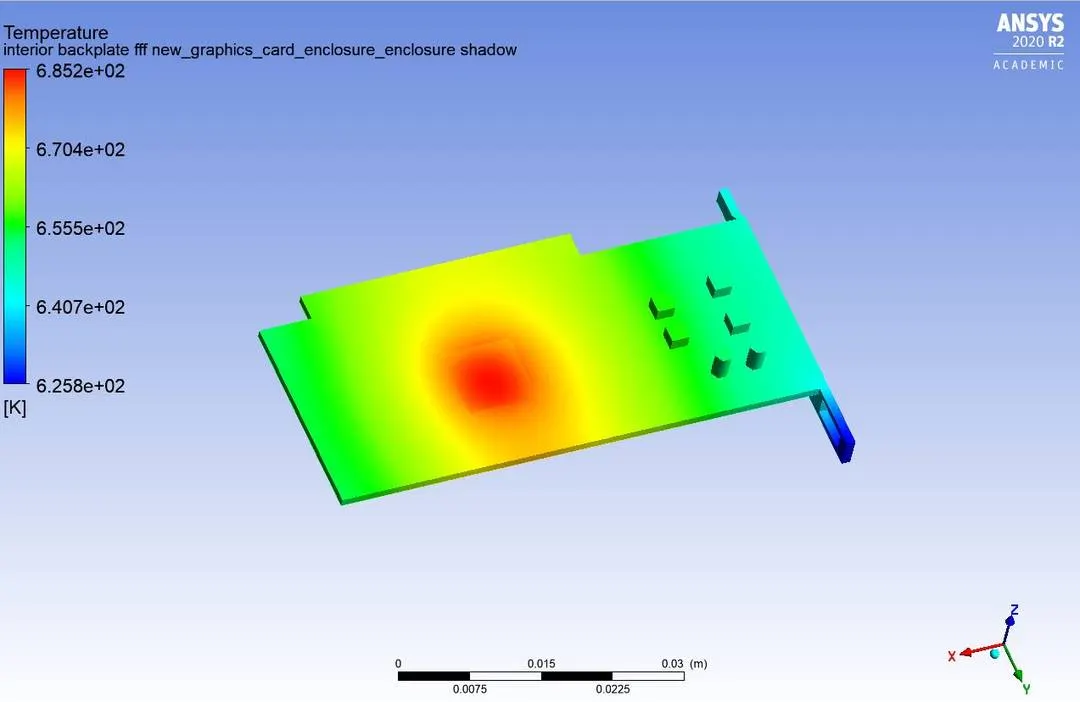
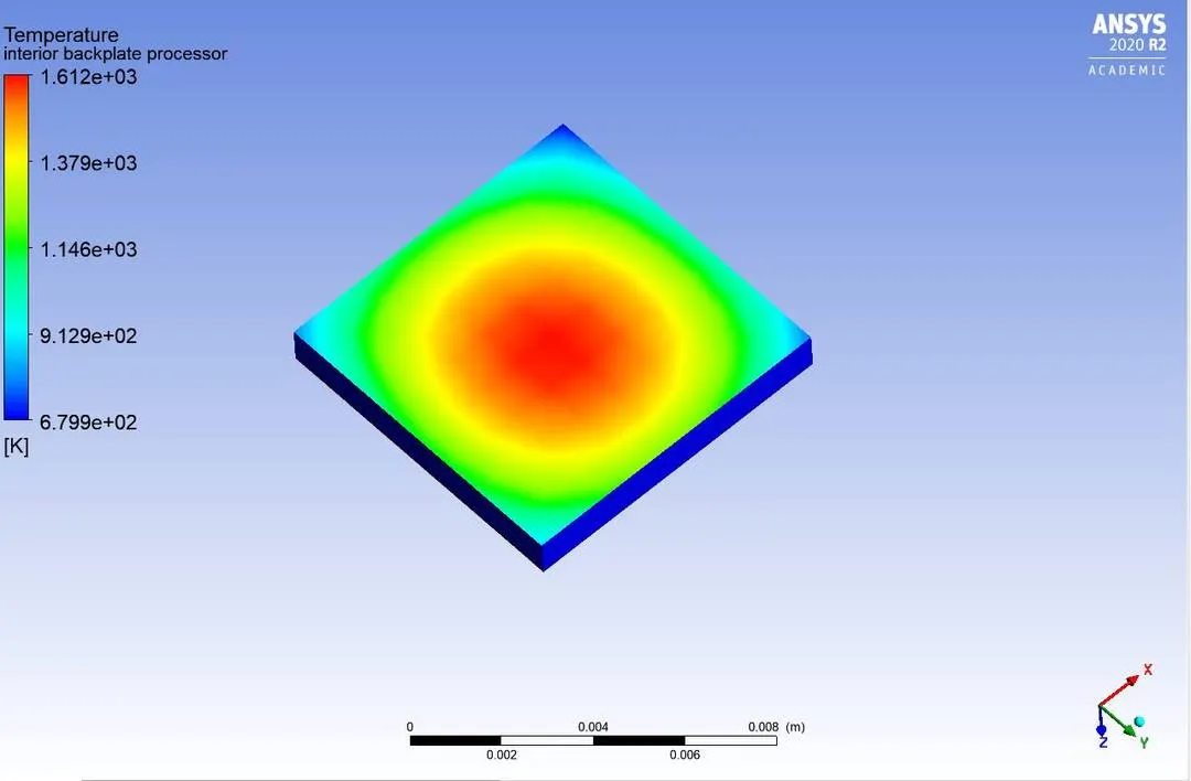
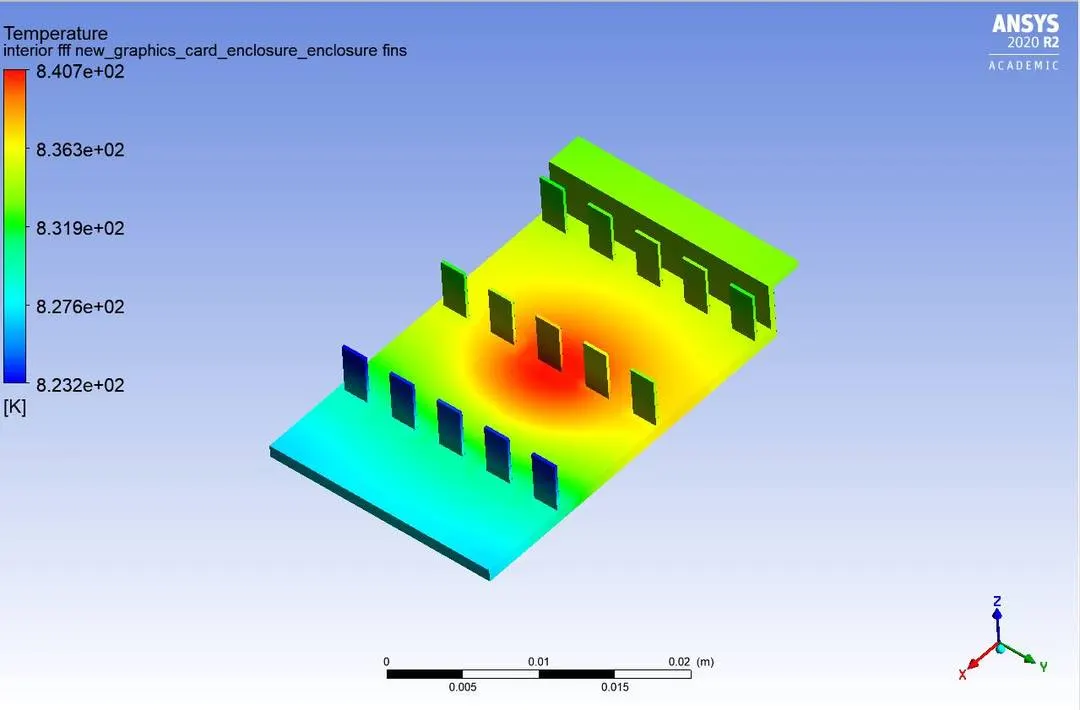
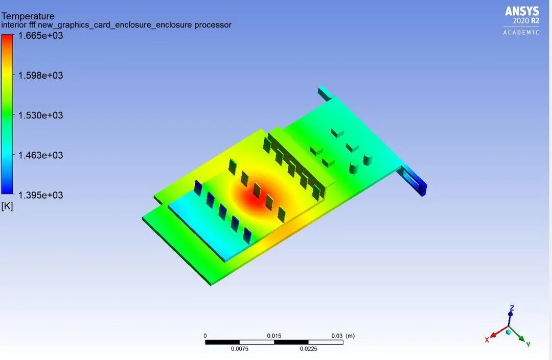
Temperature contour:

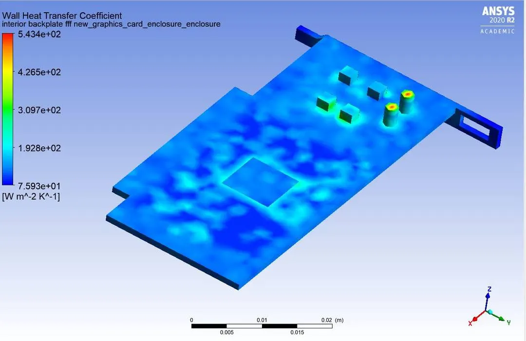
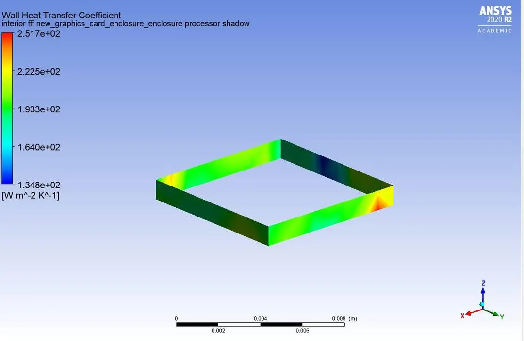
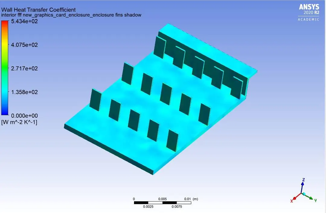
Heat transfer coefficient:

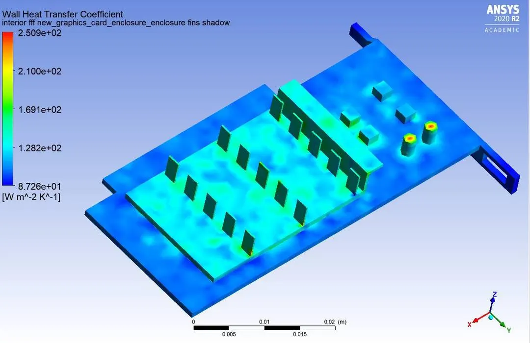
Velocity plane:

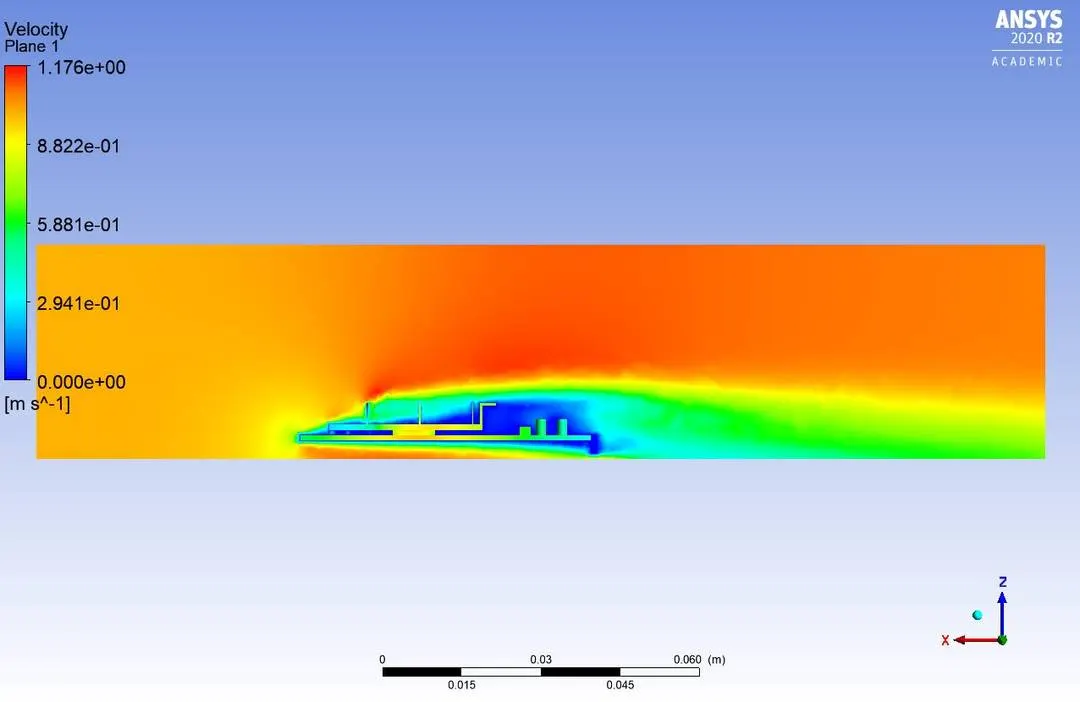
Temperature plane:

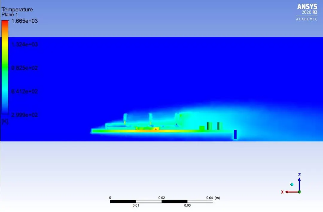
wall heat transfer coefficient plane:

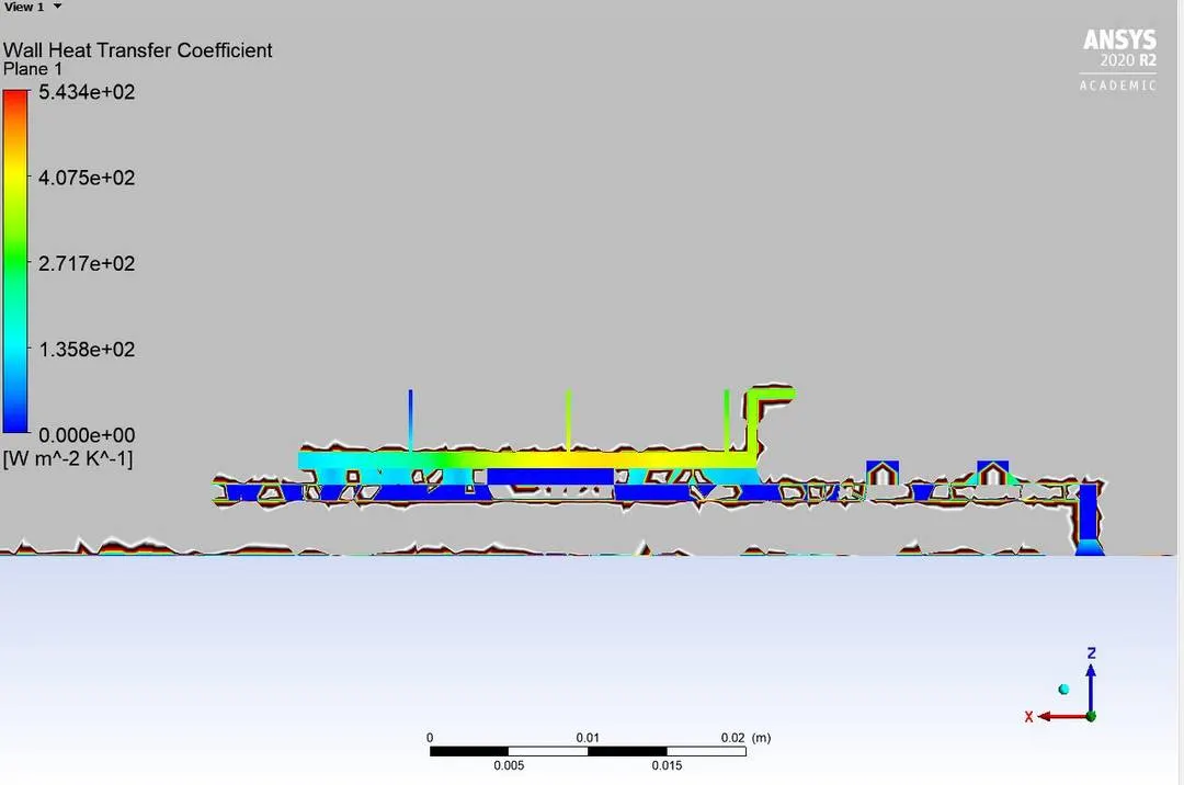
Temperature plot:

Hotspot area:

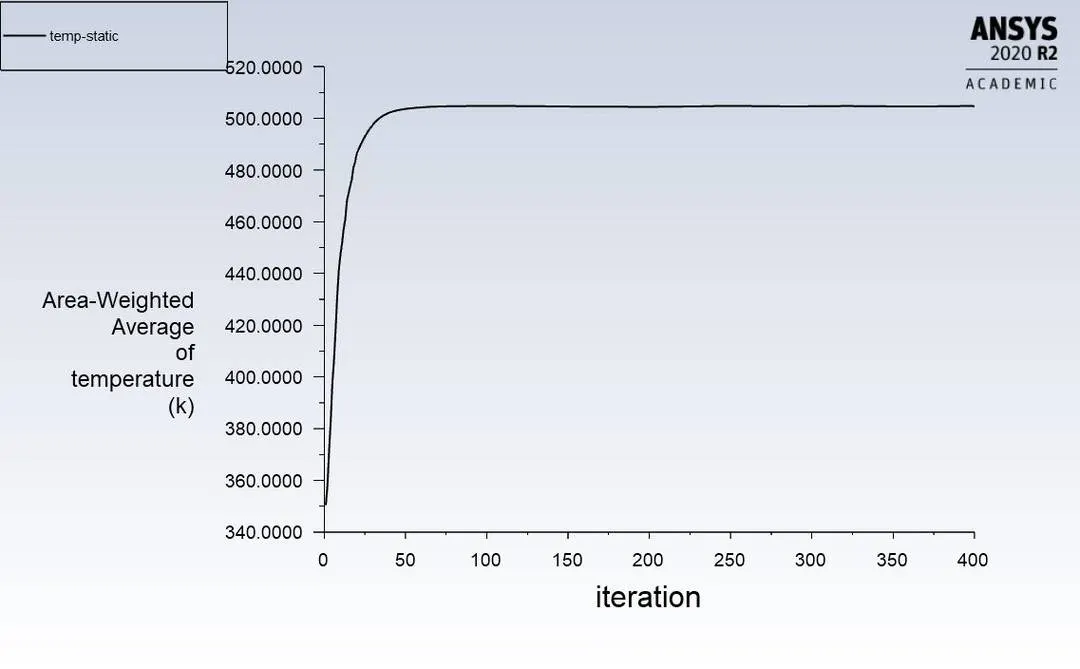
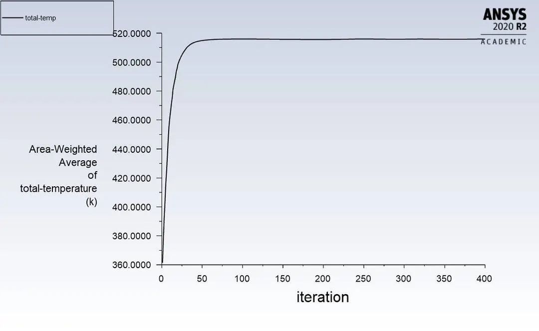
Case 3: Refined case v=3 m/s

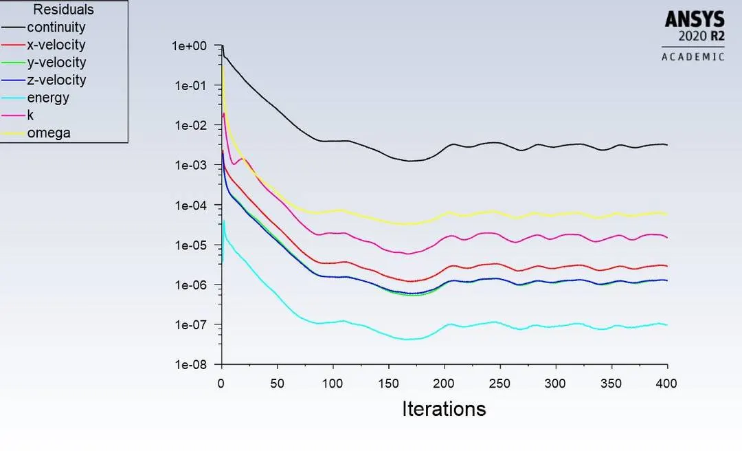
Residuals: soluton is converged

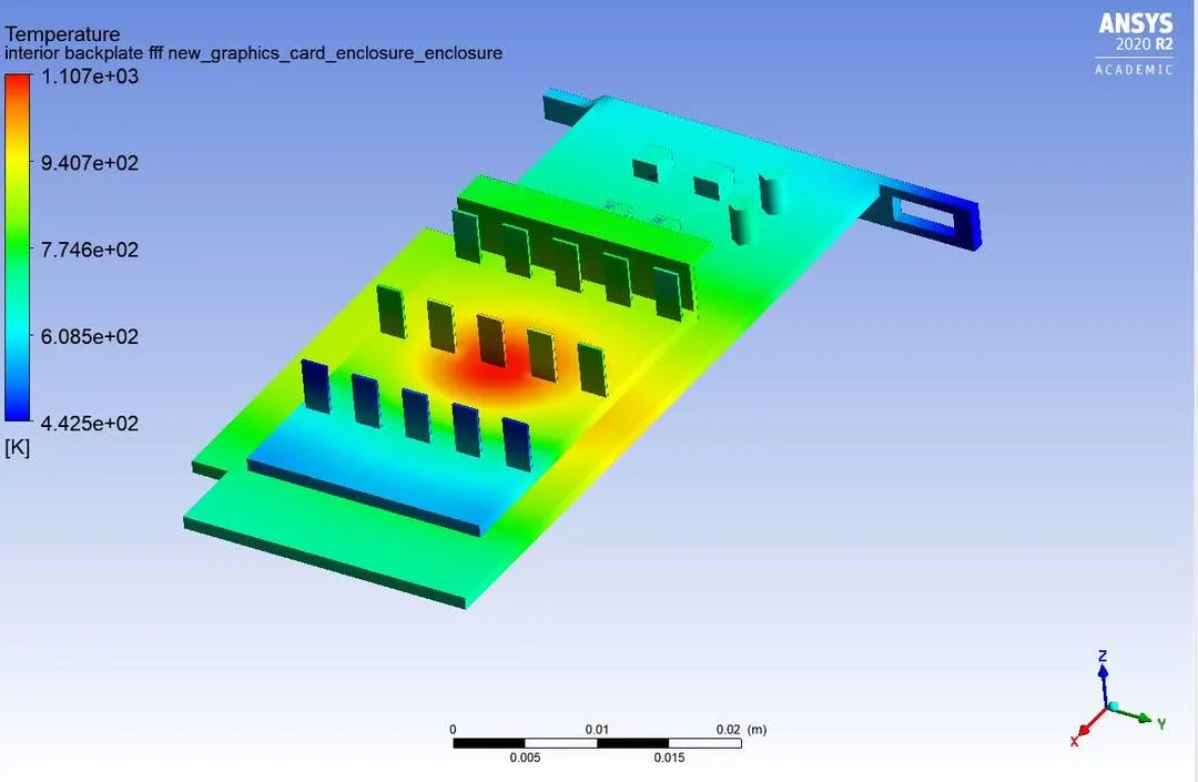
Temperature contours:

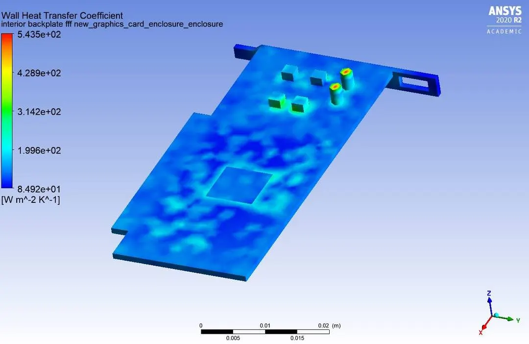
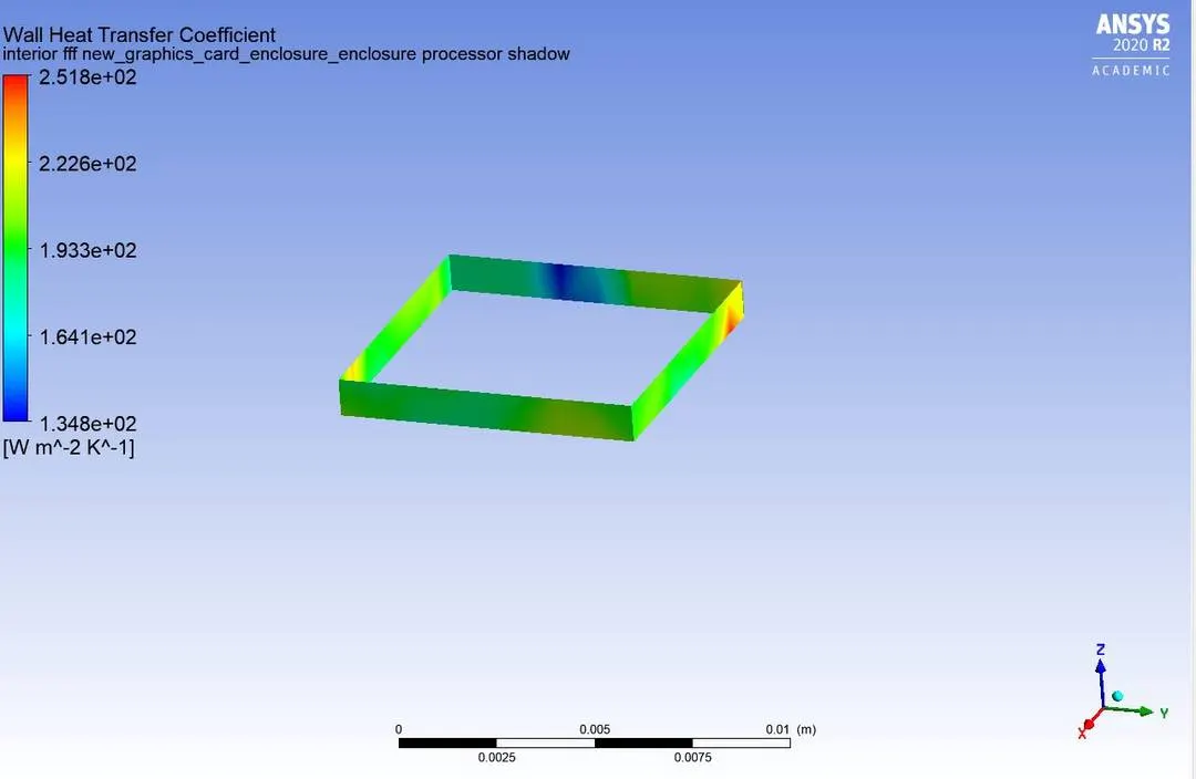
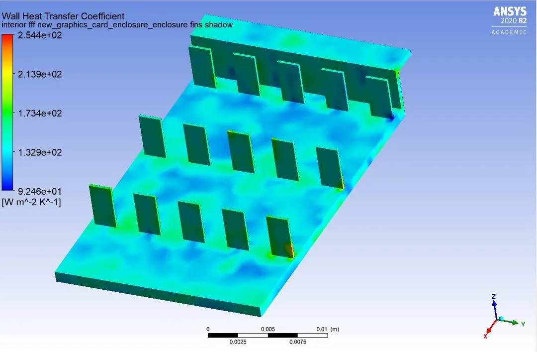
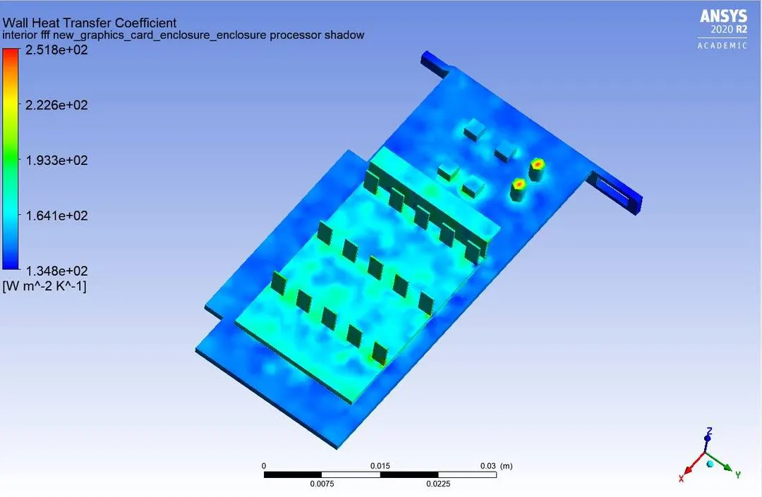
Heat transfer coeffcient:

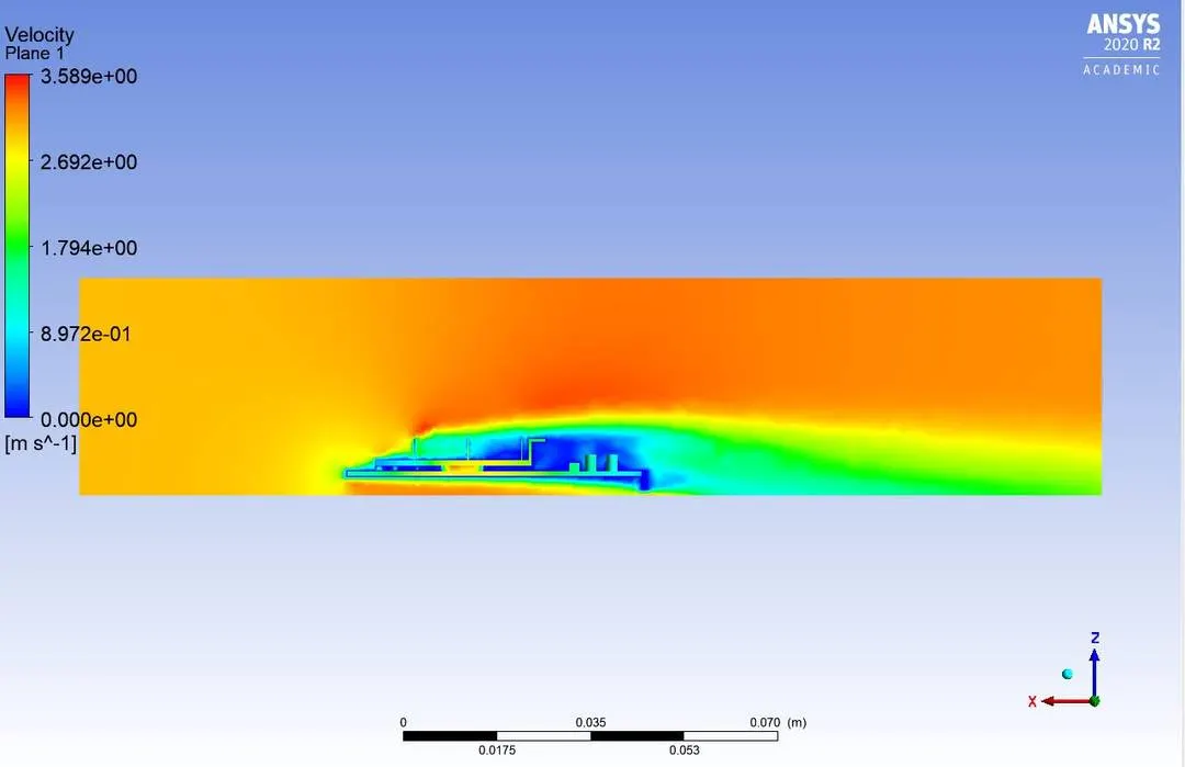
Velocity plane:

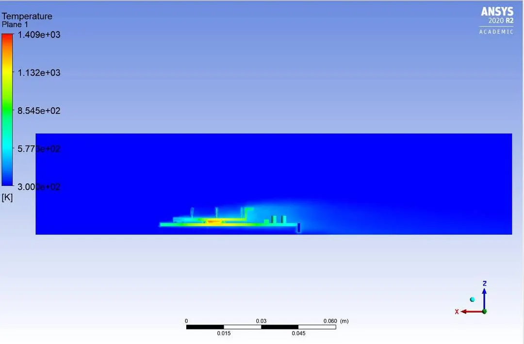
Temperature plane:

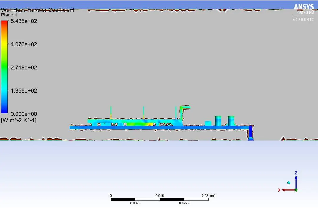
wall heat transfer coefficient:

Temperature plot:

Hotspot areas:

Case 4: Refined mesh v=5 m/s

Residuals: soluton is converged

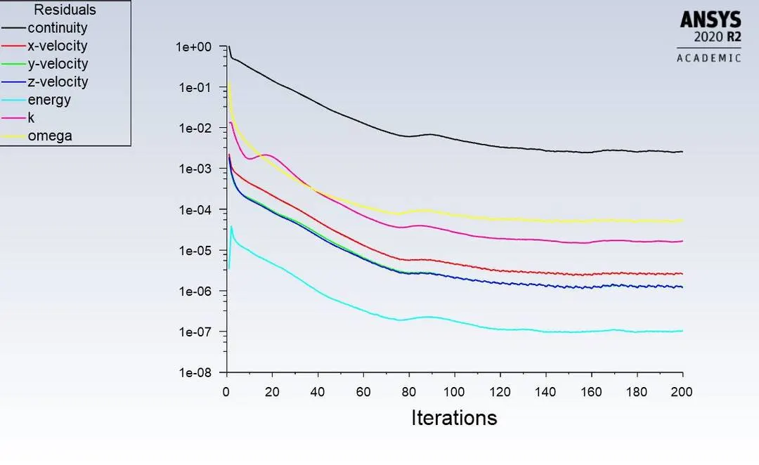
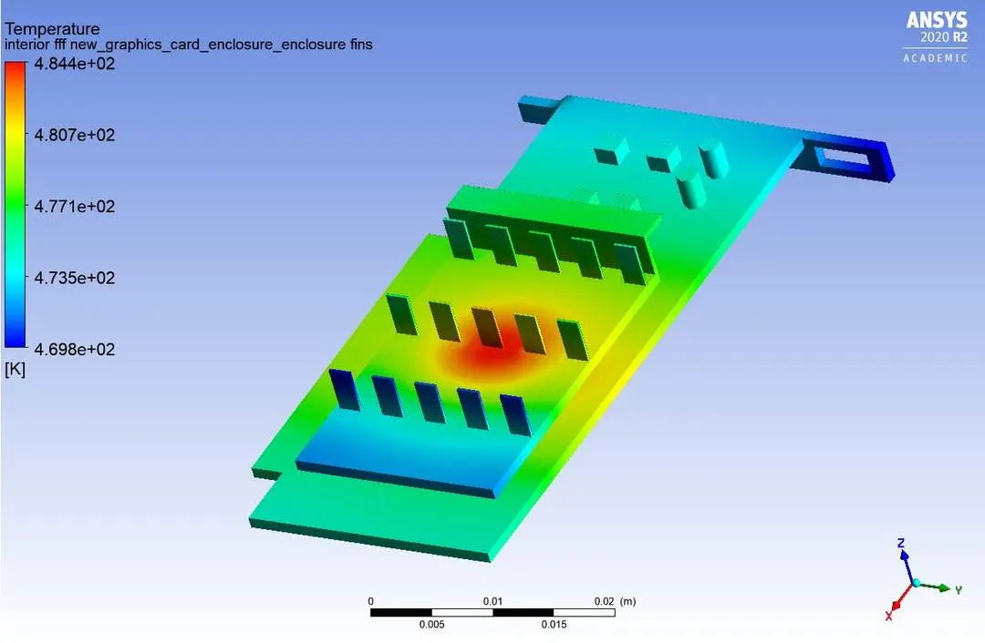
Temperature contour:

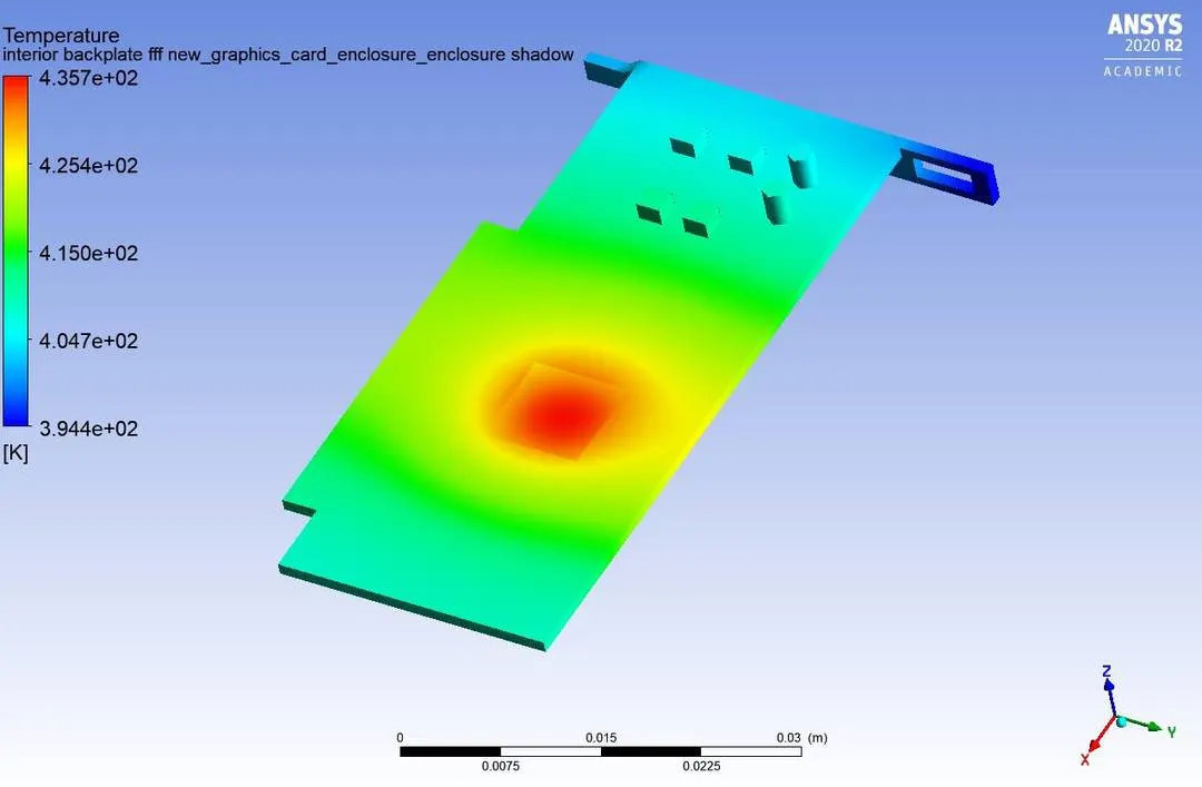
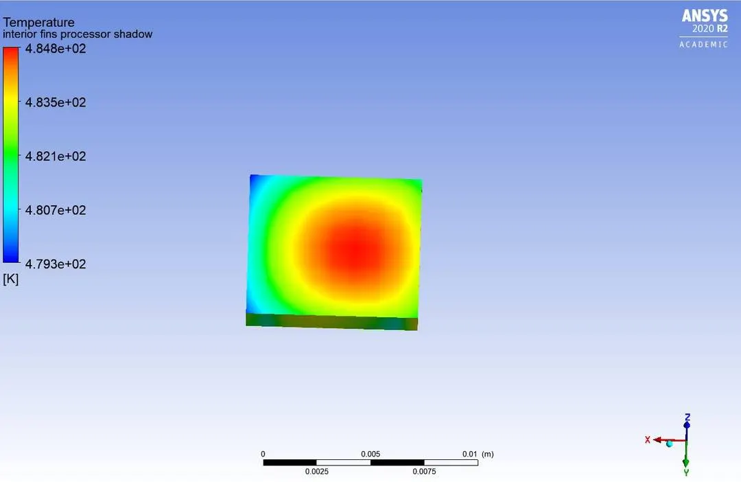
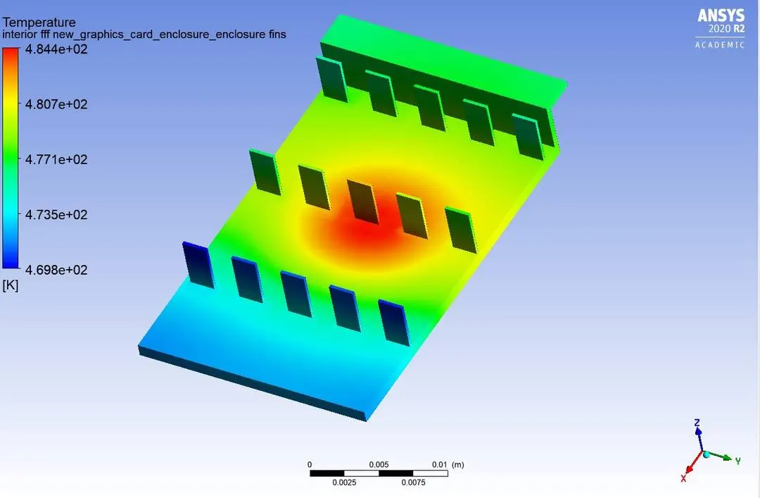
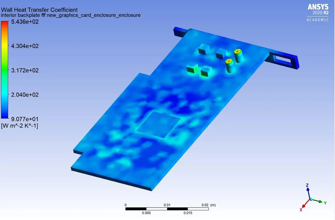
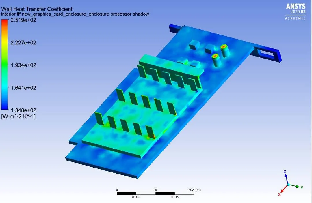
Heat transfer Coefficient:

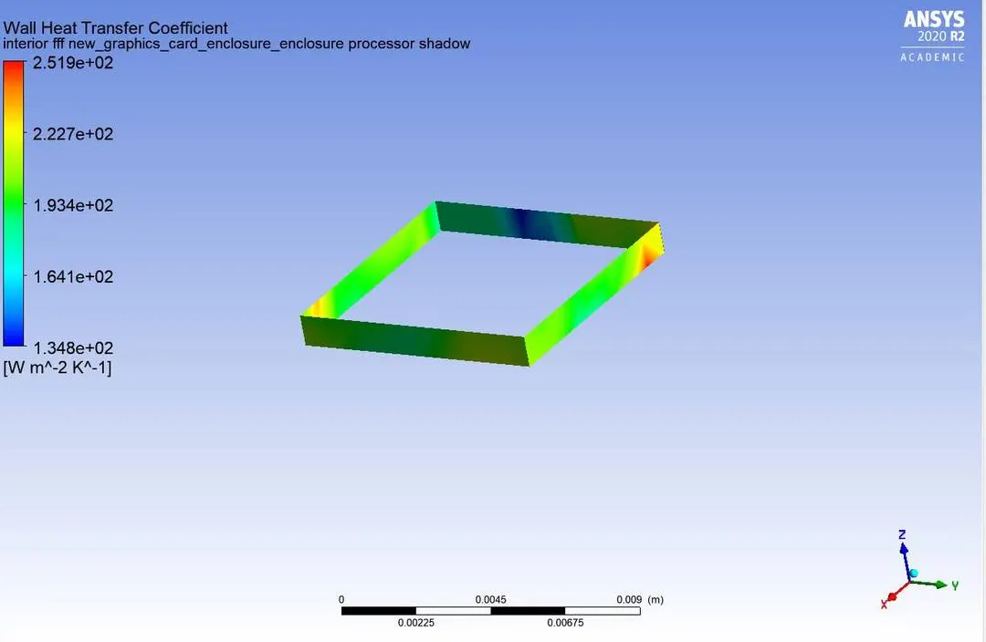
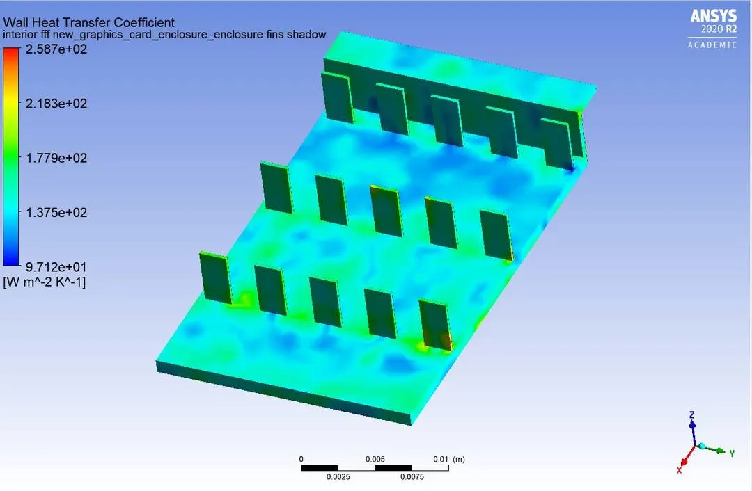
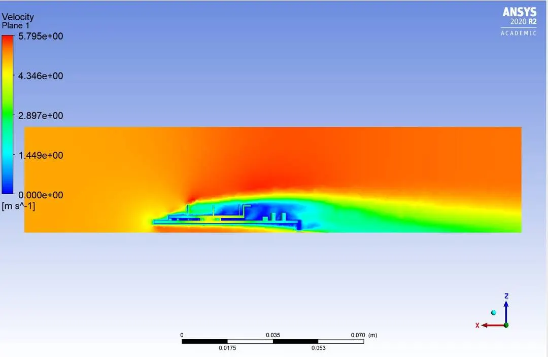
Velocity plane:

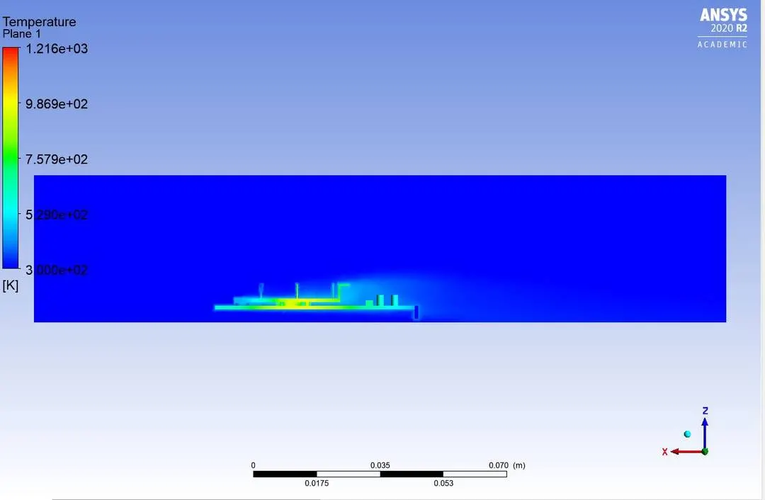
Temperature plane:

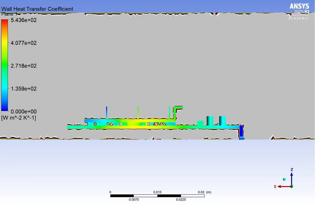
wall heat transfer coefficient:

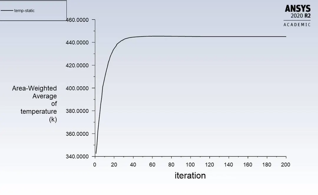
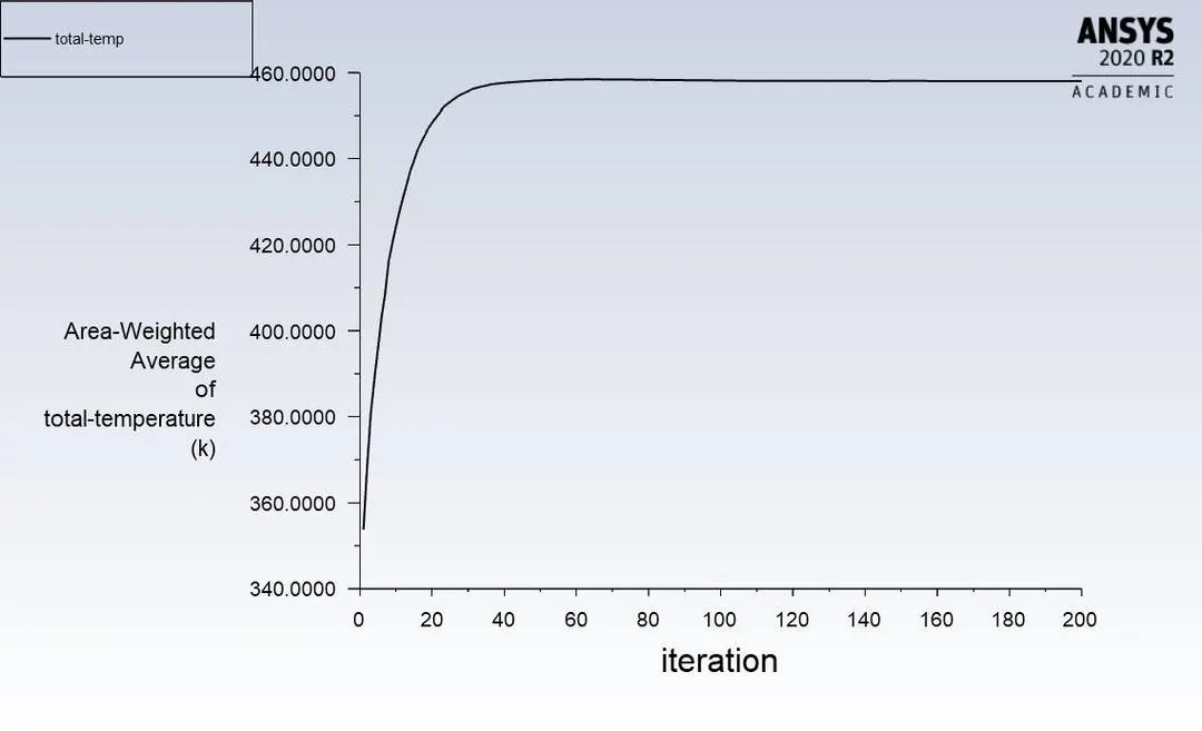
Temperature plot:

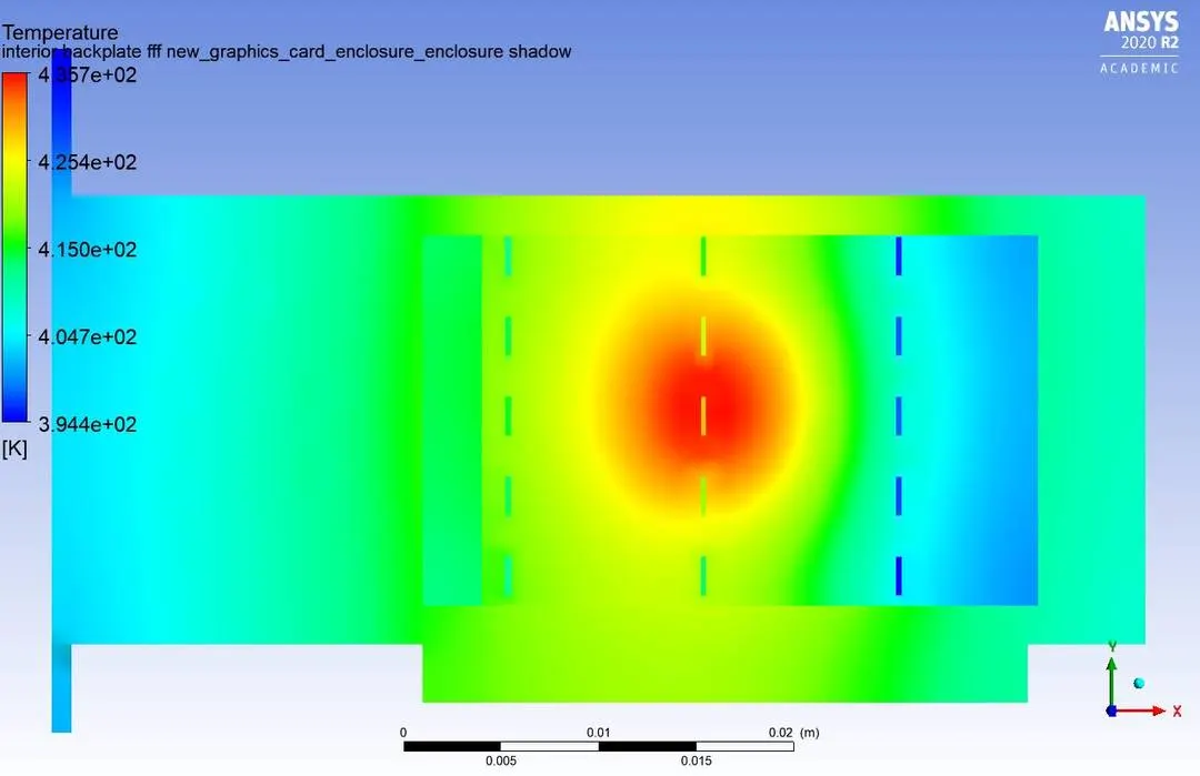
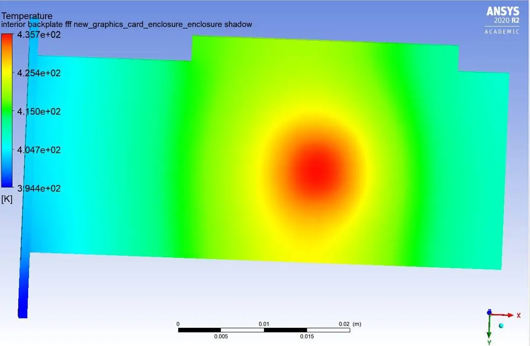
Hotspot areas:

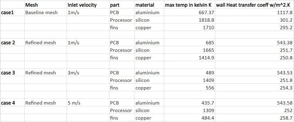
Results for all cases

Discussions:

Reason for choosing mesh settings:

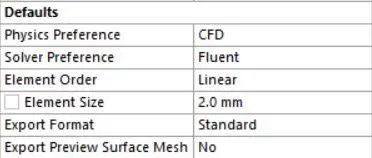
• The coarse mesh size or the baseline mesh is of 2mm of element size which pretty much capture phsyics but there are some parts where we needed refinement.
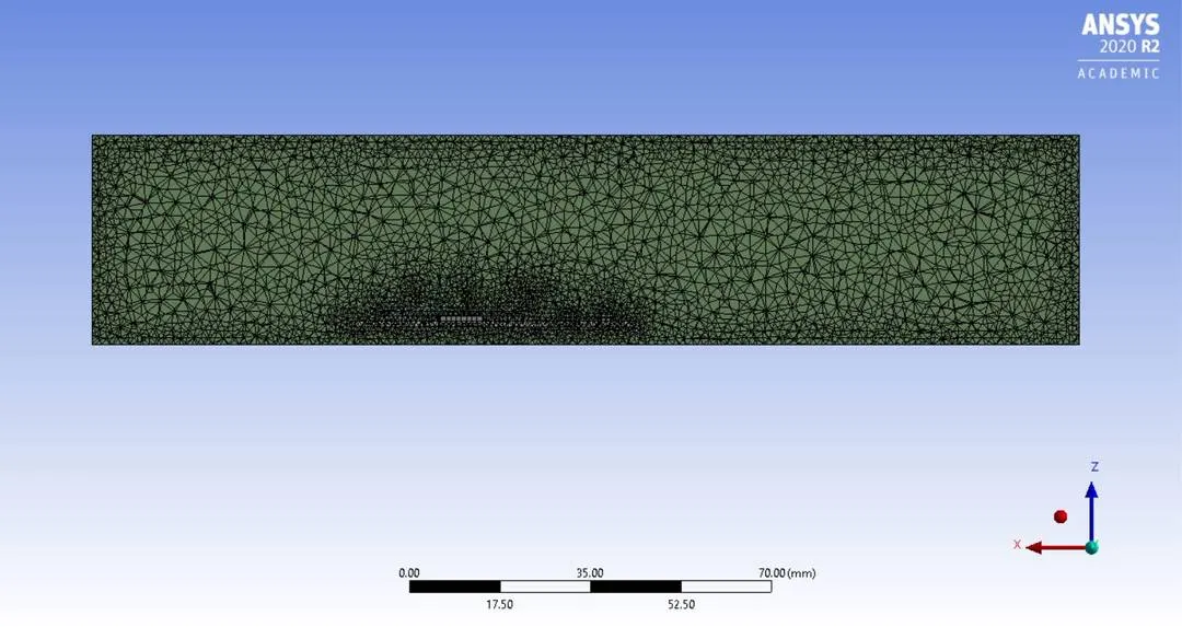
• In refined mesh settings we are mostly interested in refining the zones where in proper refinement is not done or to increase the mesh settings.
• Major refinement is done at the fins and pcb as fins are major part through which heat is shredded.
• for fins a body sizing of 1mm is taken and the same is followed for pcb.
• Element size of 1.7 mm is taken for the main mesh settings.

Note : residual plots shows the convergence of solution for all cases.

Conclusions and inferences:

• The Residuals in all cases has converged and in one case for v=3m/s there was a similar pattern of small waves which can be neglected as major part of the solution is converged.
• The Fin material is chosen as copper since it is a good conductor of heat and shreds heat in a faster pace.
• A 30 watt power consuming graphic processor is chosen since most of the graphic card processor range from 15-65 watts and its obvious that upon load the mean fluctation of power consumption will be a range of 30 watts.
• The source term generates heat and conducts through the fins and pcb and convects through the side wall of the processor.
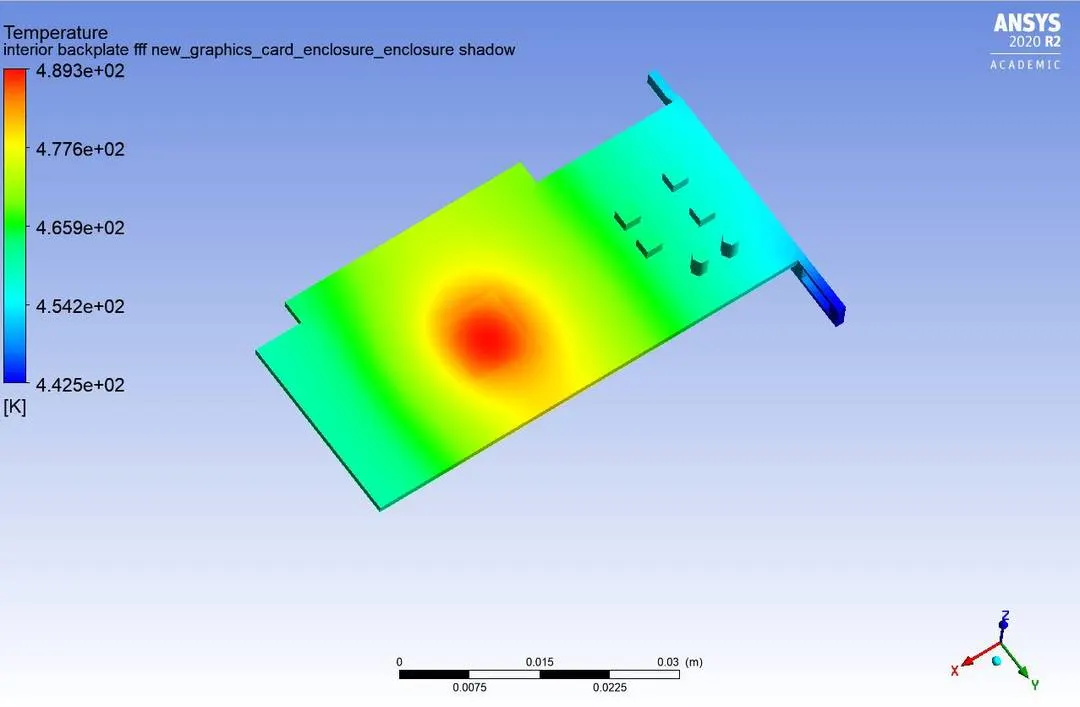
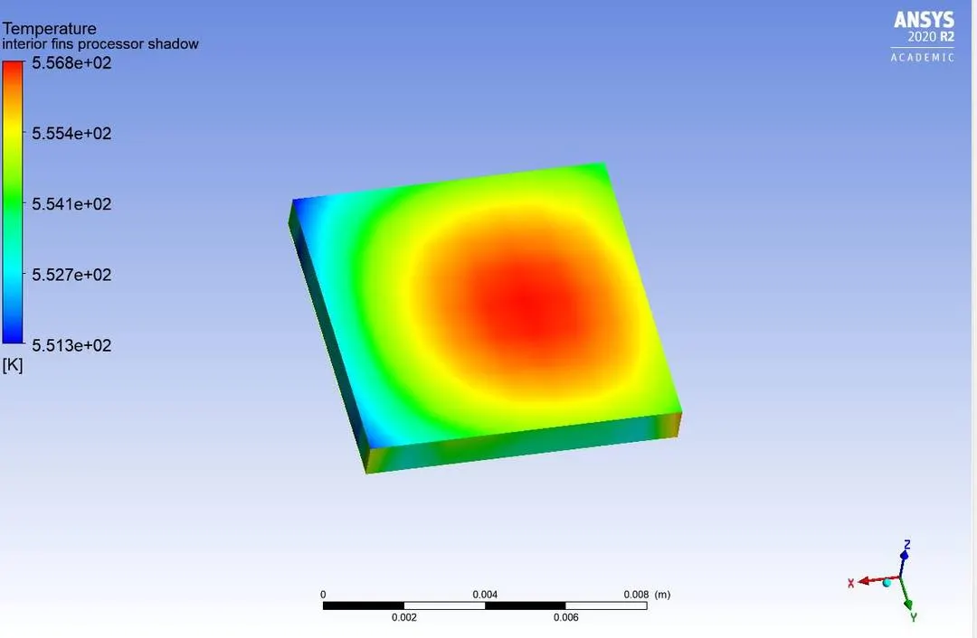
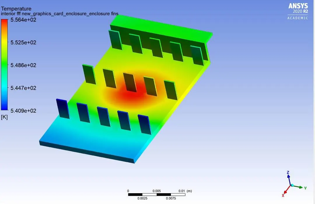
• We can observe from the results table that as the velocity of flow increases the maximum temperature of fins, processor and PCB decreases.
• Wall heat transfer coefficient somehow does not change a lot but remains low according the heat generated and the reason for such values might be the heat flux.
• Heat transfer coefficient for the PCB is highest since the surface area is more.
• As the velocity increase the heat transfer coefficient increases, the increase might be a little but this is enough to check the physics and a better understading can be obtained by much more refined mesh.
• Biot number can be increased by chosing the pcb board with less thermal conductivity(k), in this project the aluminium is not a good material to pick with but aluminum better explains the physics.
• Potential hotspots are near the adjacent wall of processor i.e on the top of fins and PCB as the heat generated is 468750000 watt/m^3 so the immediate contact areas will have major hotspots.'
• As the velocity increases the reynolds number increases and the flow strike the fins and the velocity is obstructed which causes small recirculation areas is such cases the fins design can be changed a bit to decrease recirculation areas.