Week 11 - Simulation of Flow through a pipe in OpenFoam
Aim: To create a MATLAB program to generate a computational mesh for any wedge angle and simulate the hagen poiseuille's flow for velocity and pressure drop.
Description:
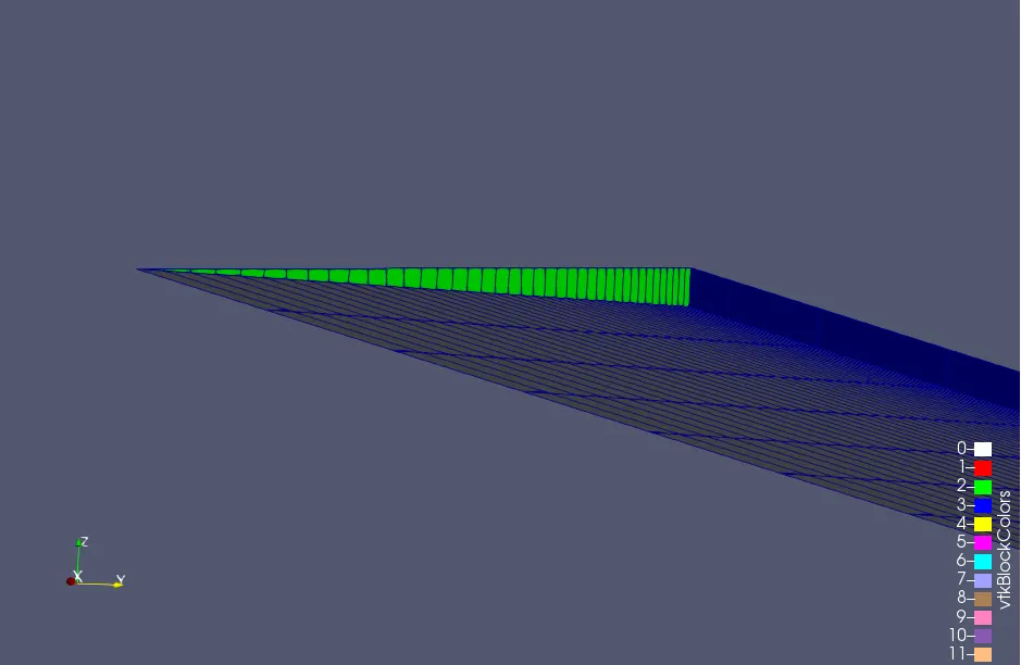
The objective is to perform a simulation of the flow through a pipe using openFoam. In this we take a wedge of angle less than 5 degrees and make a solid model. This is done through the blockMeshDict file in openfoam. The mesh is performed on the model and simulation and post processing is done to analyse the flow.
- The fluid used is water at 25 degrees celsius
- the flow is laminar
- reynolds number is 2100
- icoFoam solver is used to solve the problem in openfoam.
Hagen poiseuilles's flow equations:
Hagen poiseuille's flow is a physical law that gives the pressure drop in an incompressible and newtonian fluid. And the velocity profile for the flow through a pipe in this case. Assumptions are made in deriving the hagen poiseuilies equation regarding the dimension that the length of the pipe is much larger than its diameter (L>>D). An average velocity is calculated across the flow which is used to calculate the maximum velocity.
we derive the flow of viscous fluid through a circular pipe to find
- velocity distribution across the section
- maximum velocity
- average velocity
- ratio of maximum velocity to average velocity
- pressure drop in the pipe `Deltap=(32muoverlineuL)/(D^2)`
- the shear stress distruibution
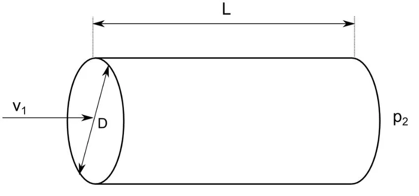
consider a pipe of length L =3 metres and diameter D=0.02metres .Dynamic viscosity of water `mu`=0.00091Ns/m^2 . The reynolds number is taken as 2100. Instead of taking the whole pipe we take a small sector of pipe this is due to the fact that a huge computational load is to be carried out while simulating for the entire pipe and by this we can save time due to axi-symmetry nature.
Hydrodynamic entrance length:
The hydrodynamic entrance region refers to the area of the pipe where the fluid entering the pipe develops a velocity profile due to the viscous forces inside the interior wall of the pipe. The region has non uniform flow. The fluid enters a pipe at a uniform velocity and the fluid particles at the wall stop completely due to no slip condition. Due to viscous forces the adjacent layers to the wall slows down so the flow at the centre is a maximum and gradually decreses as we move to the walls, by this the mass is conserved
The layer in which the shearing forces are significant is called the boundary layer
fig1. Developing velocity profile of fluid in a pipe
.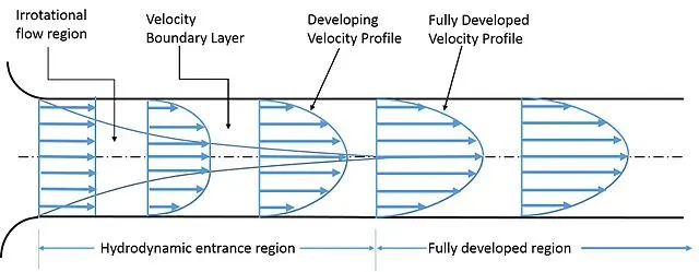
As in the figure there are two regions to concentrate i.e the hydrodynamic entrance region and the fully developed region.
As the fluid enters the boundary layers increases in thickness and gradually increases in thickness over the length. the velocity profile start generating after fluid enters into the entrance region where the domination of viscous forces can be seen and gradually the shear at the boundaries are decreased.
Shear Stress (`tau`): shear stress is highest at the pipe inlet and boundary layer thickness is the least shear stress decreases in the direction of flow so the pressure drop is highest at the inlet.
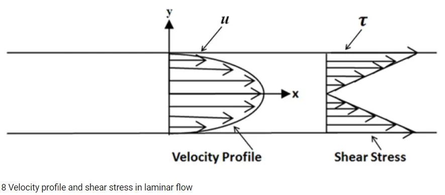
Hydrodynamic fully developed velocity profile Laminar flow: `(delu(r,x))/(delx)=0; u=u(r)`
hydrodynamic Entrance length for laminar flow: `Le=0.06*Re*D`
average velocity V_avg= `-R^2/(8mu)(dp)/(dx)`
maximum velocity V_max= 2*V_avg
Reynolds number `Re=(rhoVavgD)/(mu)`
calculating analytical solution values for fluid flow:
- Reynolds number: `Re=(rhoVavgD)/(mu)` `implies2100=(1000*Vavg*0.02)/(0.00091)impliesVavg=0.095m/s`
- Maximum velocity at the centre : `Vmax=2*Vavg implies2*0.095=0.1911m/s`
- hydrodynamic entrance length : `Le=0.06*Re*D implies0.06*2100*0.02implies2.52m`
- Total length for profile Lt=3m
- pressure drop across the pipe from Hp eqns : `Deltap=(32muVavgL)/(D^2)implies(32*0.0091*0.095*3)/(0.02^2)implies20.748kPa`
- kinematic pressure difference : `DeltaPk=(Deltap)/(rho)=20.748/1000=0.020748`
- velocity profile at any location wrt to radial direction: `u(r)=2Vavg(1-(r^2)/(R^2))`
- kinematic viscosity `nu=mu/rho implies0.00091/1000implies0.00000091 m^2/s`
Matlab code:
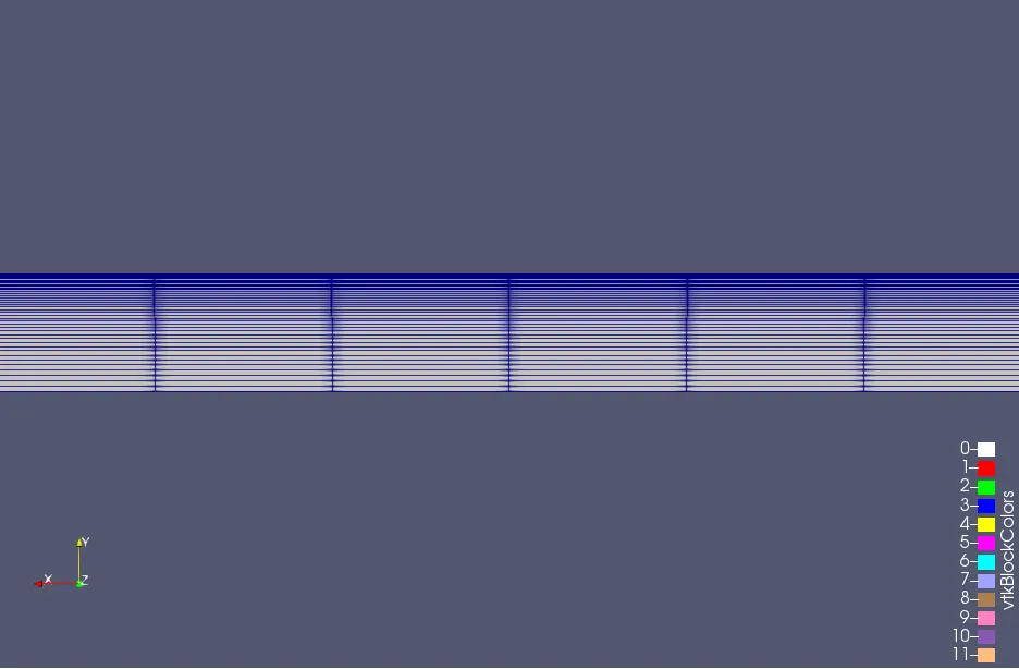
The code is written to print a text file as output to the input variables . This automatically generates a computational mesh for any wedge angle and grading schemes and stored in blockmeshDict file
clear all
close all
clc

%blockmesh file
Re=2100;
rho=1000;%kg/m^3
nu= 0.00091;%dynamic viscosity kine=dyna/rho
D=0.02;
r=D/2;
L_e = 0.06*Re*D;
L=3;
%hp eqns
v_avg = (r*nu)/(rho*D);
v_max = 2*v_avg;
dp = (32*nu*v_avg*L)/(D^2);%hagen poiseulles pressure drop
kinematic_p= dp/(rho);

th=4;
%meshing
mx=200;
my=40;
mz=1;
fx=1;%grading factor f
fy=0.2;
fz=1;

%vertices
v0=[0 0 0];
v1=[0 r*cosd(th/2) r*sind(th/2)];
v2=[0 r*cosd(th/2) -r*sind(th/2)];
v3=[3 0 0];
v4=[3 r*cosd(th/2) r*sind(th/2)];
v5=[3 r*cosd(th/2) -r*sind(th/2)];

header1='/*--------------------------------*- C++ -*----------------------------------*\'
header2=' =========             	|'
header3=' \\  	/   F ield     	| OpenFOAM: The Open Source CFD Toolbox'
header4='  \\	/   O peration 	| Website:  https://openfoam.org'
header5='   \\  /	A nd       	| Version:  8'
header6='	 \\/ 	M anipulation  |'
header7='\*---------------------------------------------------------------------------*/'
header8='FoamFile'
header9='{'
header11='version 	2.0;'
header12='format  	ascii;'
header13='class   	dictionary;'
header14='object  	blockMeshDict;'
header15='}'
header16='// * * * * * * * * * * * * * * * * * * * * * * * * * * * * * * * * * * * * * //'


f1=fopen('blockMeshDict','w')
fprintf(f1,'%sn',header1)
fprintf(f1,'%sn',header2)
fprintf(f1,'%sn',header3)
fprintf(f1,'%sn',header4)
fprintf(f1,'%sn',header5)
fprintf(f1,'%sn',header6)
fprintf(f1,'%sn',header7)
fprintf(f1,'%sn',header8)
fprintf(f1,'%sn',header9)
fprintf(f1,'%sn',header11)
fprintf(f1,'%sn',header12)
fprintf(f1,'%sn',header13)
fprintf(f1,'%sn',header14)
fprintf(f1,'%sn',header15)
fprintf(f1,'%sn',header16)

fprintf(f1,'convertToMeters 1;nn')

fprintf(f1,'verticesn')
fprintf(f1,'(n')
fprintf(f1,'t (%d %d %d)n',0,0,0)
fprintf(f1,'t (%d %d %d)n',0,r*cosd(th/2),r*sind(th/2))
fprintf(f1,'t (%d %d %d)n',0,r*cosd(th/2),-r*sind(th/2))
fprintf(f1,'t (%d %d %d)n',3,0,0)
fprintf(f1,'t (%d %d %d)n',3,r*cosd(th/2),r*sind(th/2))
fprintf(f1,'t (%d %d %d)n',3,r*cosd(th/2),-r*sind(th/2))
fprintf(f1,');nn')

fprintf(f1,'blocksn')
fprintf(f1,'(n')
fprintf(f1,'t hex (0 3 5 2 0 3 4 1) (200 40 1) simpleGrading (1 0.2 1)')
fprintf(f1,');nn')

fprintf(f1,'edgesn')
fprintf(f1,'(n')
fprintf(f1,'t arc 1 2 (0 0.01000 0)')
fprintf(f1,'t arc 4 5 (3 0.01000 0)')
fprintf(f1,');nn')

fprintf(f1,'boundaryn')
fprintf(f1,'(n')
fprintf(f1,'t inletn')
fprintf(f1,'t {n')
fprintf(f1,'t type patch;')
fprintf(f1,'t facesn')
fprintf(f1,'(n')
fprintf(f1,'(0 1 2 0)')
fprintf(f1,');n')
fprintf(f1,'t }n')

fprintf(f1,'t outletn')
fprintf(f1,'t {n')
fprintf(f1,'t type patch;')
fprintf(f1,'t facesn')
fprintf(f1,'(n')
fprintf(f1,'(3 5 4 3)')
fprintf(f1,');n')
fprintf(f1,'t }n')

fprintf(f1,'t topwalln')
fprintf(f1,'t {n')
fprintf(f1,'t type wall;')
fprintf(f1,'t facesn')
fprintf(f1,'(n')
fprintf(f1,'(1 4 5 2)')
fprintf(f1,');n')
fprintf(f1,'t }n')

fprintf(f1,'t frontn')
fprintf(f1,'t {n')
fprintf(f1,'t type wedge;')
fprintf(f1,'t facesn')
fprintf(f1,'(n')
fprintf(f1,'(0 2 5 3)')
fprintf(f1,');n')
fprintf(f1,'t }n')

fprintf(f1,'t backn')
fprintf(f1,'t {n')
fprintf(f1,'t type wedge;')
fprintf(f1,'t facesn')
fprintf(f1,'(n')
fprintf(f1,'(0 3 4 1)')
fprintf(f1,');n')
fprintf(f1,'t }n')

fprintf(f1,'t axisn')
fprintf(f1,'t {n')
fprintf(f1,'t type empty;')
fprintf(f1,'t facesn')
fprintf(f1,'(n')
fprintf(f1,'(0 3 3 0)')
fprintf(f1,');n')
fprintf(f1,'t }n')
fprintf(f1,');n')


fprintf(f1,'mergePatchPairs')
fprintf(f1,'t {n')
fprintf(f1,');nn')
fprintf(f1,'header16')

fclose(f1)
BlockmeshDict file
/*--------------------------------*- C++ -*----------------------------------*\
  =========                 |
  \\      /  F ield         | OpenFOAM: The Open Source CFD Toolbox
   \\    /   O peration     | Website:  https://openfoam.org
    \\  /    A nd           | Version:  8
     \\/     M anipulation  |
\*---------------------------------------------------------------------------*/
FoamFile
{
    version     2.0;
    format      ascii;
    class       dictionary;
    object      blockMeshDict;
}
// * * * * * * * * * * * * * * * * * * * * * * * * * * * * * * * * * * * * * //

convertToMeters 1;

vertices
(
    (0 0 0)//v0
    (0 0.009994 0.000349)//v1
    (0 0.009994 -0.000349)//v2
    (3 0 0)//v3
    (3 0.009994 0.000349)//v4
    (3 0.009994 -0.000349)//v5

);

blocks
(
    hex (0 3 5 2 0 3 4 1) (200 40 1) simpleGrading (1 0.2 1)
);

edges
(
    arc 1 2 (0 0.01000 0)
    arc 4 5 (3 0.01000 0)
);

boundary
(
    inlet
    {
        type patch;
        faces
        (
            (0 1 2 0)
        );
    }
    outlet
    {
        type patch;
        faces
        (
            (3 5 4 3)
        );
    }
    topwall
    {
        type wall;
        faces
        (
            (1 4 5 2)
        );
    }
    front
    {
        type wedge;
        faces
        (
            (0 2 5 3)
        );
    }
    back
    {
        type wedge;
        faces
        (
            (0 3 4 1)
        );
     }
     axis
    {
        type empty;
        faces
        (
            (0 3 3 0)
        );
    }
);

mergePatchPairs
(
);

// ************************************************************************* //
velocity file:
/*--------------------------------*- C++ -*----------------------------------*\
  =========                 |
  \\      /  F ield         | OpenFOAM: The Open Source CFD Toolbox
   \\    /   O peration     | Website:  https://openfoam.org
    \\  /    A nd           | Version:  8
     \\/     M anipulation  |
\*---------------------------------------------------------------------------*/
FoamFile
{
    version     2.0;
    format      ascii;
    class       volVectorField;
    object      U;
}
// * * * * * * * * * * * * * * * * * * * * * * * * * * * * * * * * * * * * * //

dimensions      [0 1 -1 0 0 0 0];

internalField   uniform (0 0 0);

boundaryField
{
    inlet
    {
        type            fixedValue;
        value           uniform (0.095 0 0);
    }

    outlet
    {
        type            zeroGradient;
    }

    topwall
    {
        type            noSlip;
    }
    front
    {
        type            wedge;
    }
    back
    {
        type            wedge;
    }
    axis
    {
        type            empty;
    }
}

// ************************************************************************* //
pressure:
/*--------------------------------*- C++ -*----------------------------------*\
  =========                 |
  \\      /  F ield         | OpenFOAM: The Open Source CFD Toolbox
   \\    /   O peration     | Website:  https://openfoam.org
    \\  /    A nd           | Version:  8
     \\/     M anipulation  |
\*---------------------------------------------------------------------------*/
FoamFile
{
    version     2.0;
    format      ascii;
    class       volScalarField;
    object      p;
}
// * * * * * * * * * * * * * * * * * * * * * * * * * * * * * * * * * * * * * //

dimensions      [0 2 -2 0 0 0 0];

internalField   uniform 0;

boundaryField
{
    inlet
    {
        type            zeroGradient;
    }

    outlet
    {
        type            fixedValue;
        value           uniform 0;
    }

    topwall
    {
        type            zeroGradient;
    }

    front
    {
        type            wedge;
    }

    back
    {
        type            wedge;
    }

    axis
    {
        type            empty;
    }
}


// ************************************************************************* //
Control Dict:
/*--------------------------------*- C++ -*----------------------------------*\
  =========                 |
  \\      /  F ield         | OpenFOAM: The Open Source CFD Toolbox
   \\    /   O peration     | Website:  https://openfoam.org
    \\  /    A nd           | Version:  8
     \\/     M anipulation  |
\*---------------------------------------------------------------------------*/
FoamFile
{
    version     2.0;
    format      ascii;
    class       dictionary;
    location    "system";
    object      controlDict;
}
// * * * * * * * * * * * * * * * * * * * * * * * * * * * * * * * * * * * * * //

application     icoFoam;

startFrom       startTime;

startTime       0;

stopAt          endTime;

endTime         50;

deltaT          0.01;

writeControl    timeStep;

writeInterval   20;

purgeWrite      0;

writeFormat     ascii;

writePrecision  6;

writeCompression off;

timeFormat      general;

timePrecision   6;

runTimeModifiable true;


// ************************************************************************* //
Transport properties:
/*--------------------------------*- C++ -*----------------------------------*\
  =========                 |
  \\      /  F ield         | OpenFOAM: The Open Source CFD Toolbox
   \\    /   O peration     | Website:  https://openfoam.org
    \\  /    A nd           | Version:  8
     \\/     M anipulation  |
\*---------------------------------------------------------------------------*/
FoamFile
{
    version     2.0;
    format      ascii;
    class       dictionary;
    location    "constant";
    object      transportProperties;
}
// * * * * * * * * * * * * * * * * * * * * * * * * * * * * * * * * * * * * * //

nu              [0 2 -1 0 0 0 0] 0.00000091;


// ************************************************************************* //
Explnation for the simulation :
The initial and boundary conditions are taken in the 0 folder in which we specify the average velocity and the pressure in resprective U and P files. Now change the control settings in the control Dict file for courant number <1 .
The solver used is IcoFoam. It is chosen because of our flow characteristics which we are simulating. since its a hagen poiseullies flow which is incompressible and newtonian fluid so IcoFoam is best suitable as it solves for incompressible flow incorporating navier stokes equation .
The transport properties kinematic viscosity is chosen as 0.0000009 m^2/s.
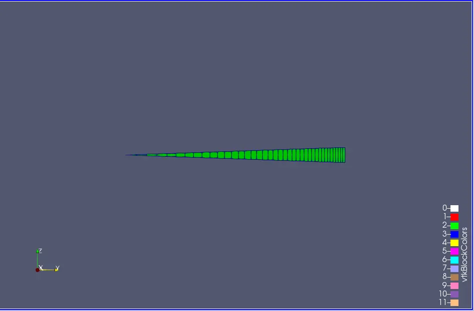
Mesh using blockMesh:
Post Processing:
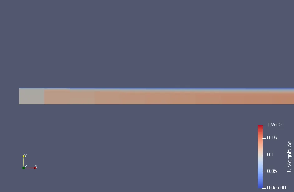
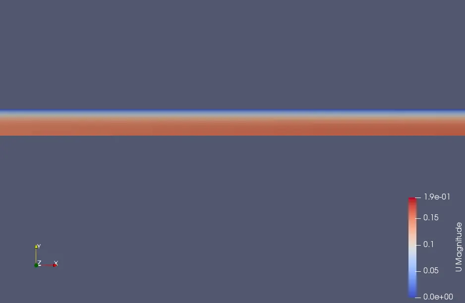
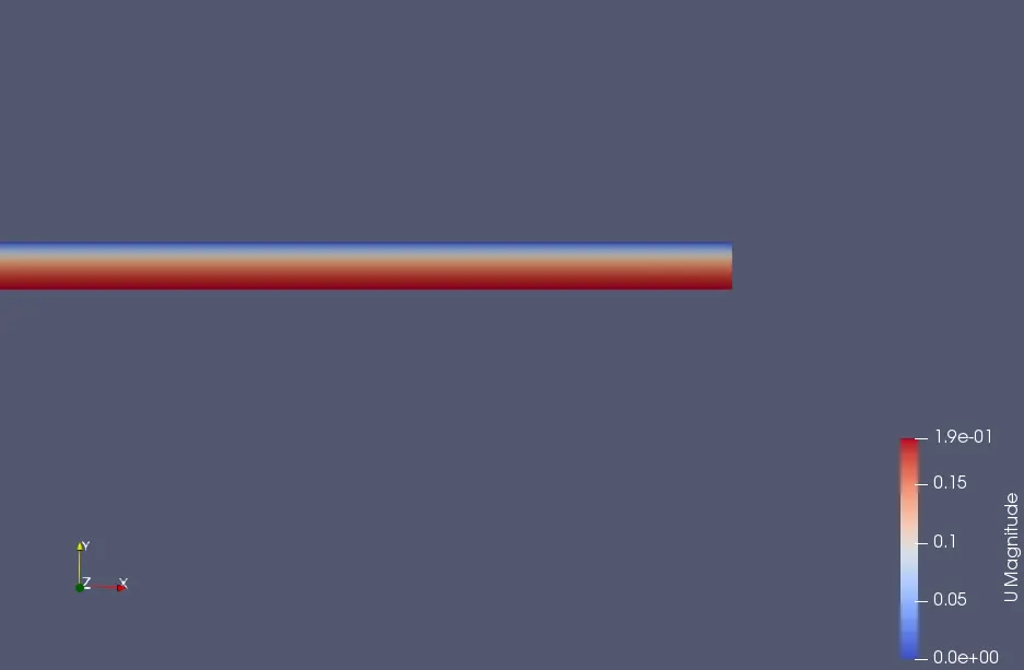
Post processing is done using ParaFoam which open ups paraview in which we can alter the orientaiin and see the flow. The flow parameter analysed are velocity, pressure and shear stress distribution across the pipe.
velocity distribution along the pipe:
At inlet:
Intermediate velocity:
final velocity at exit:
Plots:
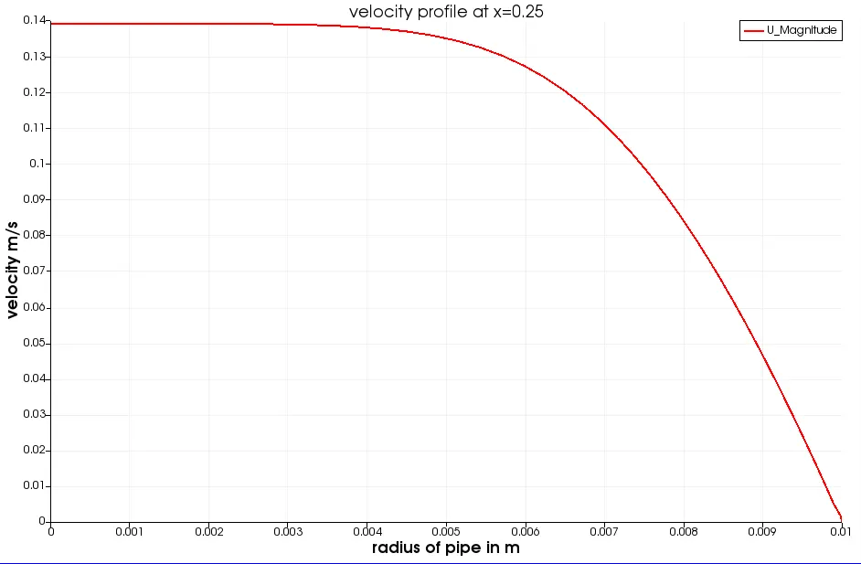
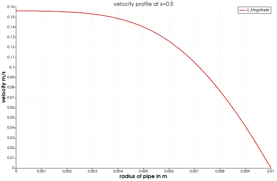
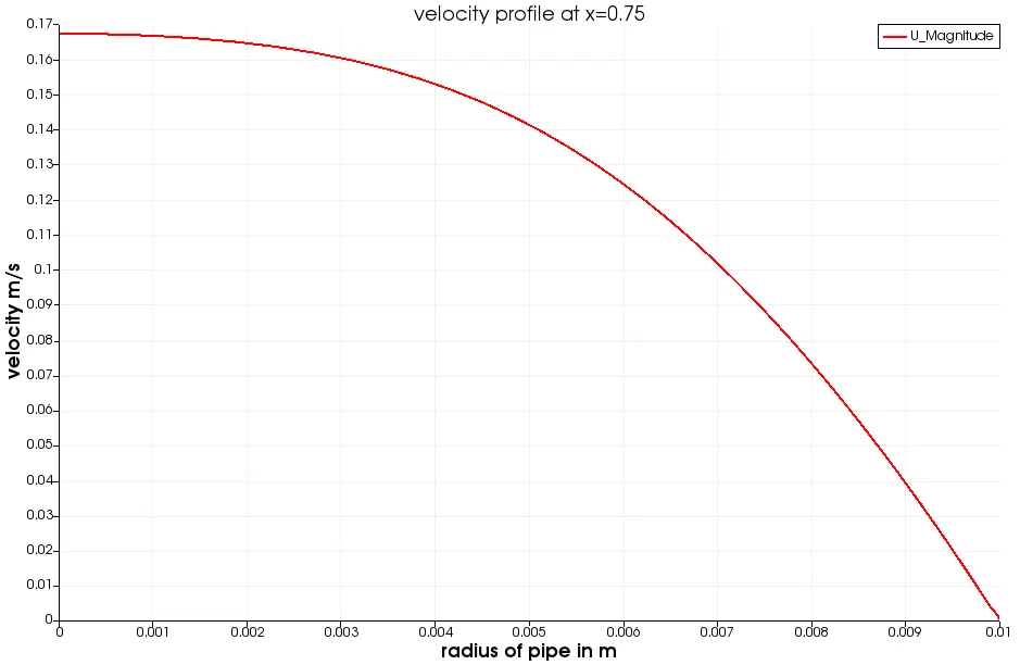
velocity profile plot along radial direction with length along x axis:
velocity profile along x=0.25m:
velocity profile along x=0.5m:
velocity profile along x=0.75m:
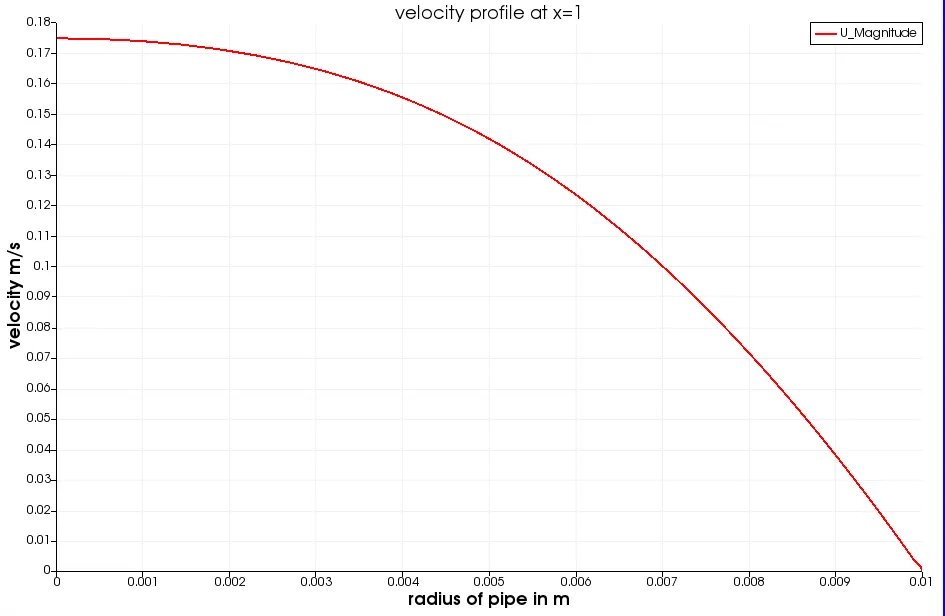
velocity profile along x=1m:
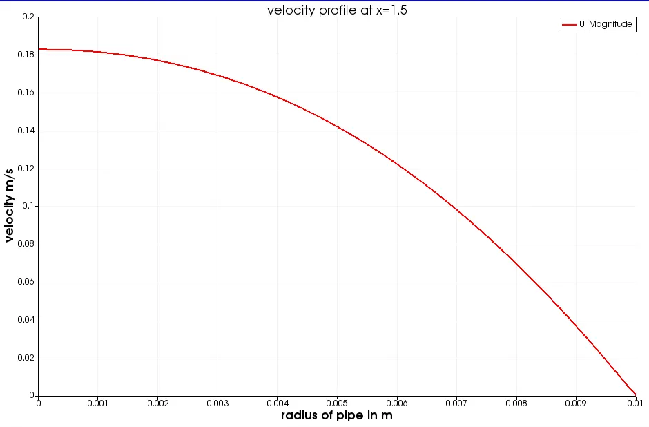
velocity profile along x=1.5m:
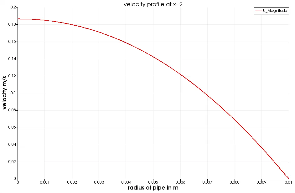
velocity profile along x=2m:
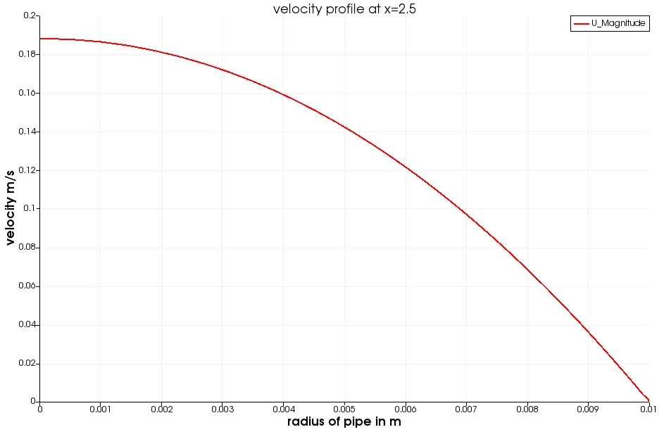
velocity profile along x=2.5m:
velocity profile along x=3m:
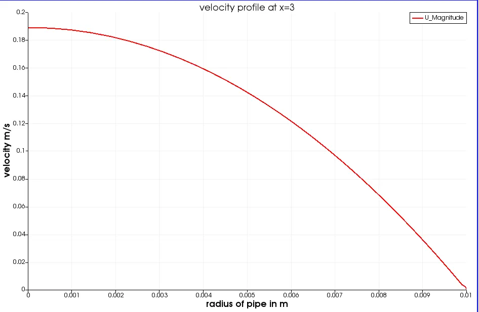
Explanation for velocity plots:
- The fluid enters with an average velocity of 0.095m/s
- from the above plots there is a clear transition of velocity field along x direction at x=0.25,0.5,0.75,1,1.5,2,2.5,3
- Along x direction the velocity increases from 0.14m/s at inlet to 0.19m/s at outlet.
- The hydeodynamic length extends till 2.52 m where we can see a fully developed flow
- The maximum velocity Vmax is 0.19m/s which is in alignment with the Hagen poiseulles flow velocity
Pressure:
Pressure distribution:
At inlet:
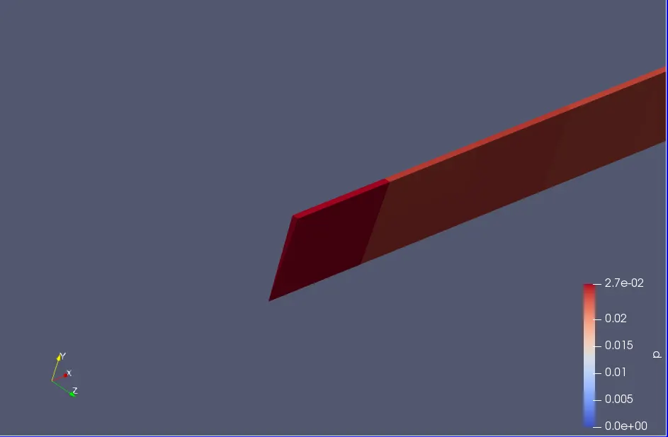
outlet pressure:
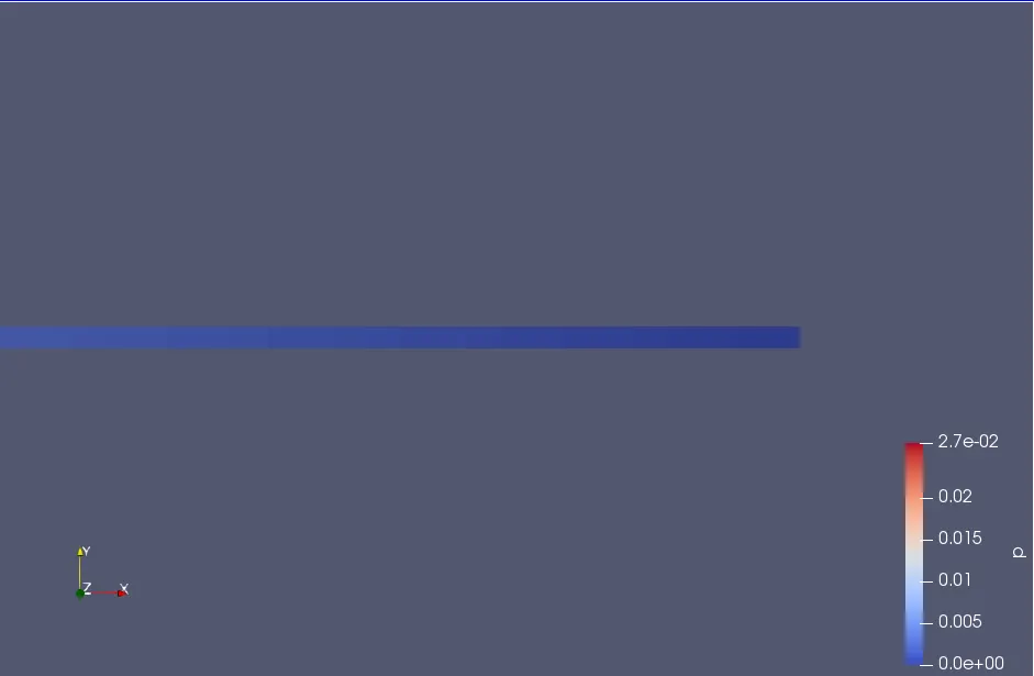
plots for Pressure:
Pressure distribution along x axis length of pipe:
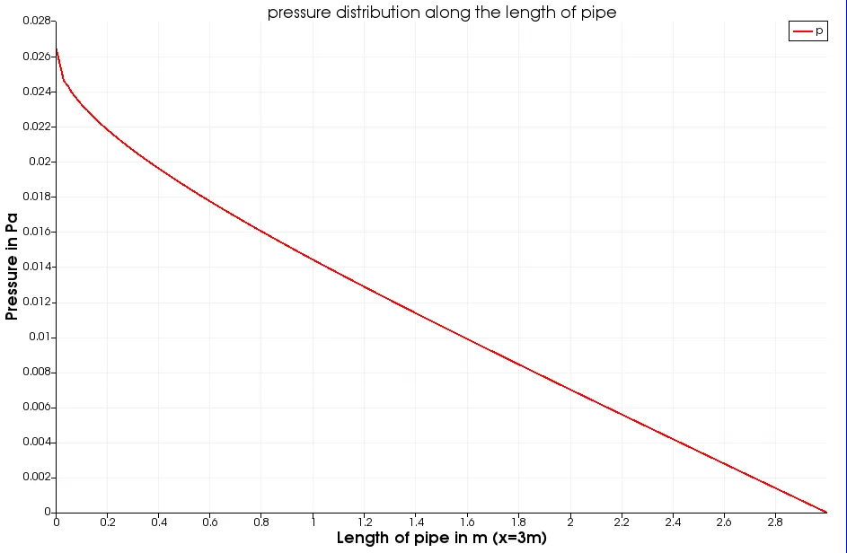
The inlet pressure is 0.0267 N/m^2 and outlet is absolute zero.
shear stress:
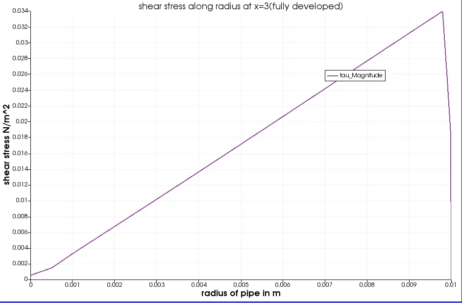
Plot of wall shear stress along radial direction at x=3m:
Explanation of shear stress plot:
- Max shear stress is 0.034 N/m^2
- The shear stress due to viscous forces are high at walls and linearly decreases at the centre.
- the formula used for computation is `tau=mu(du)/(dr)`
Results:
Hagen Poiseulles flow comaprision of results for velocity and pressure drop:
velocity max anlytical=0.1911m/s
velocity max openfoam=0.1900m/s
error in velocity 0.57%
pressure drop analytical: 0.02075 pa
pressure drop openfoam=0.02670pa
conclusion:
- Hagen poiseulles flow is computed in accordance with the assumption made to be an incompressible flow and newtonian.
- The velocity distribution simulated for the wedge is in accordance to hagen poiseulles flow.
- The pressure drop is carried out was in accordance to the Hp presssue drop.
- The wall shear stress is n accordance with analytically computed.
- The maximum velocity at the centre of pipe is justified in the plots.
- The maximum shear stress at the wall of pipe is justified in the plots.
- The drop in pressure is justified in plots.
- The three computation made for velocity , pressure and shear stress justifies the analytical and computational domain of Openfoam.