Week 9 - FVM Literature Review

Finite Volume Method (FVM):

Finite volume method is a discretized method for approximation the system of partial differential equations. FVM method is used to solve the governing equation which are in intergral form.

In FVM method we write equations for a volume instead of writing equation for a single point as in the finite difference method. Small volumes of grids are considered and on each finite small piece of volume. We apply the governing equations and then integrate the equation over the whole volume. By this we can calculate variables like temperature,pressure, velocity at the centroid of each control volume.The flow should satisfy the governing equation which constitute the basics of mass conservation. To convert the volume intergral to surface we need Gauss divergence therorem and then descritize the form.we have blocks of small control volume which have information about the variables and are separated by walls /faces

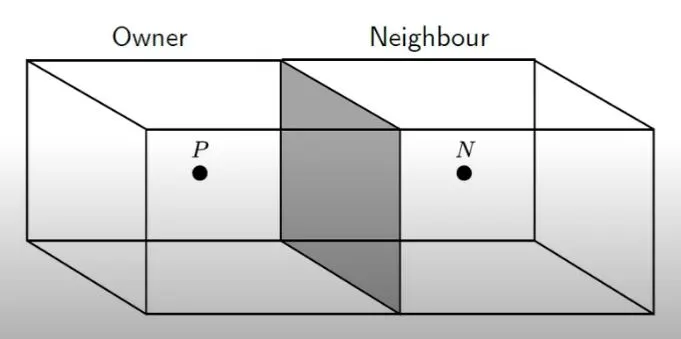
The flow variables are stored in the centroid of cell (P,N) . The linear differentiation is carried out for calculating the immediate neighbour.

Major differences

• Major differences in FDM and FVM is the consideration of cells.
• In FDM the domain on which we need to apply governing eqaution is a small point of the complete shape whereas the FVM uses small finite sized volume of the complete shape.
• By considering the FVM method we can incorporate complicated geometries to solve the problem with accuracy whereas the FDM method is not much advisable for such geometries.
• This is because the descrtization is done from point to point in FDM which takes more time and increases the error in the sytem.

Need for Interpolation schemes:

Interpolation schemes are needed to transfer the information of variables like p,T,v from one cell centroid to another cell centroid in a linear differencing schemes to calculate the values of unknown cell. The basic maths involved is differencing schemes for applications like convection-diffussion problem. The types are central, upwind and hybrid differencing scheme.

Example of 1D linear heat condution equation

lets consider the equation:

`(del)/(delx)(alpha(delT)/(delx))+S=0`

where `alpha`=thermal conductivity

T=temperature

S= source term or heat generation

take a small piece of volume

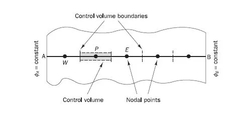
the control volume p has nodal points East E and West W.

lets integrate the governing equation over the entire body

`int_w^e[(del)/(delx)(alpha(delT)/(delx))+S]dV=0`

`int_w^e[(del)/(delx)(alpha(delT)/(delx))]dV+int_w^eSdV=0`

`int_w^e[(del)/(delx)(alpha(delT)/(delx))]Adx+int_w^eSdV=0`

after integration

`[alpha A(delT)/(delx)]_w^e+overlineSdV=0`

`alphaundersete A(delT)/(delx,e)-alphaundersetw A(delT)/(delx,w)+overlineSdV=0`

we can use taylor series approxiamation to discretize the temperature gradient term

`alphaA[(TE-TP)/(Deltax)]-alphaA[(TP-TW)/(Deltax)]+overlineSdV=0`

`(TE-TP)/(Deltax)----------------heat flux`

`overlineS-----source`

if `alpha=f(T)` then we need to descritize the alpha too using interpolation schemes.

Flux limiters:

The name flux limiter suggest that the flux or gradient schemes like spatial derivatives are bounded or limited to a partiular solution or value. They are used in higher order spatial descritization schemes to reduce the effect of uncertainities like oscillation in the solution.Flux limiters are also referred as slope limiters since the function is same that is to limit the solution gradient in this case of ID heat conduction is the heat flux term to avoid descrepencies near shock and discontinuities in the higher order schemes.