Mixing efficiency

Aim:

To set up a steady state simulation to find out the mixing effectiveness of short tee and long tee model when hot temperature inlet is at 36 degree celsius and cold inlet temperature is at 19 degree celsius.

Objective:

To use the K-epsilon and K-omega sst model to simuate the model for different momentum ratio of 2 and 4.

Case 1:

• Short mixing tee with a hot inlet velocity of 3m/s.
• Momentum ratio of 2, 4.

Case 2:

• Long mixing tee with a hot inlet velocity of 3m/s.
• Momentum ratio of 2, 4.

To make a table of comparison of following values of 2 above cases:

1. Cell count
2. Average outlet temperature
3. Number of iterations for convergence

Description:

In order to perform the steady state simulation of short tee and long tee by using different momentum ratio. The k-epsilon and k-omega model is incorporated for both the cases to check for better convergence and outlet temperature and velocity distribution along with average temperature. The perform the simulation we first mesh the model using the regular sizing which is coarse and then we decrease the mesh size to check for grid independency. After this we do the simulation by using steady state solver by using k-epsilon and k-omega turbulence model.

Cad model :

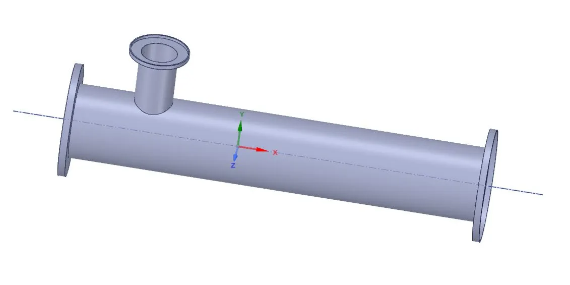
short tee:

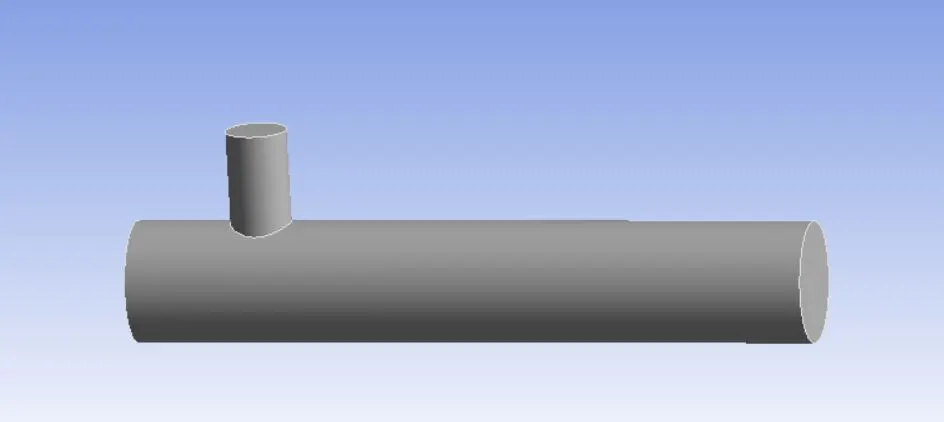
Long tee:

Boundary conditions for both k-epsilon and k-omega model:

Inlet	momentum ratio=2	momentum ratio=4
hot inlet=36 degree cesius	Vinlet x = 3 m/s	Vinlet x = 3 m/s
cold inlet=19 degree cesius	Vinlet y = 6 m/s	Vinlet y = 12 m/s

pressure outlet set to zero gauge

Theory:

K-epsilon turbulence model:

Its a high Reynolds number model. This model is a two equation model that gives the description of turbulence by means of two transport equations which are partial differential eqautions.The first transport variable is the turbulent kinetic energy (k) and the second is rate of dissipiation of turbulent kinetic energy (epsilon `epsilon`).

The model is specifically used for shear stress and recirculation flow or where the pressure gradients are small. k-epsilon turbulence model is generally used where flow does not demand to integrate the solution through the viscous sublayer and wall bounded effects are secondary.

Realizable k-epsilon model:

It provides improved prediction for the spreading rate of both planar and round jets. It also gives good results for flow involved in roation,boundary layer and strong pressure gradients. so on a whole it gives better results for complex geometries.

k -omega sst turbulence model:

Its a low reynolds number model.This model is a two equation model that gives the description of turbulence , which are partial differential eqautions.The first variable is the turbulent kinetic energy (k) and the second is specific rate of dissipiation of turbulent kinetic energy (omega `omega`).

This model takes elliptical wall behavior meaning that it has an inherent nature of being able to communicate with the wall and actually has Dirchlet(no slip) boundary condition. Commonly used for situations where the flow demands integrating through the viscous sublayer which includes heat transfer, calculation of aerodynamic drag and flow with adverse pressure gradients.

SETUP:

Now setting up for case 1 is needed to understand both the models:

workflow:

• Mesh
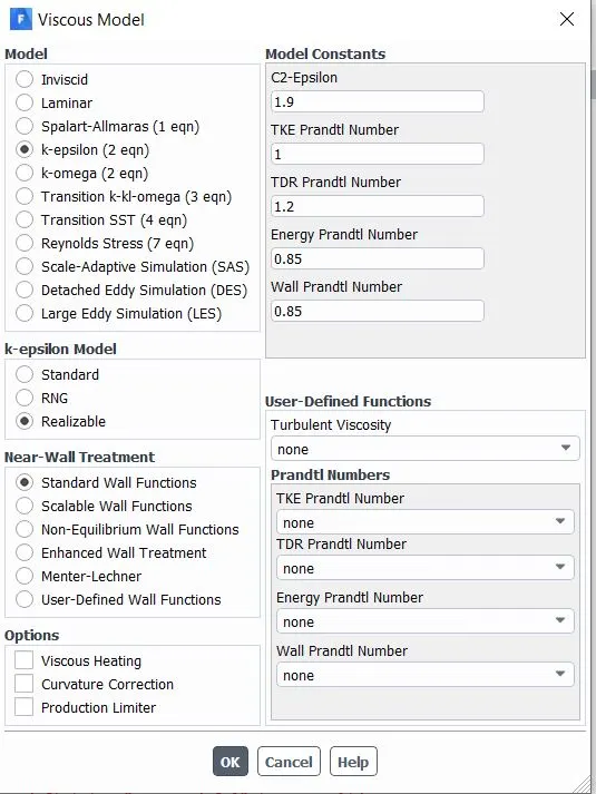
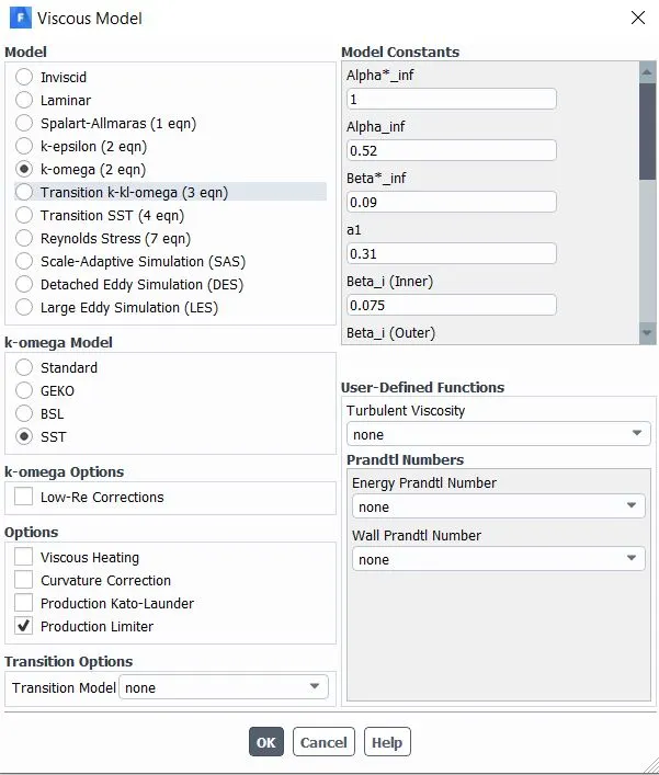
• Setup-physics-viscous flow-k-epsilon model or k-omega model
• boundary conditions for MR_2,MR_4.
• create definitions for output plot for residual, temperature and standard deviation.
• initiliaze the solution
• calculate for x number of iterations.

Different setup models :

Case 1: short tee MR=2

k-epsilon model:

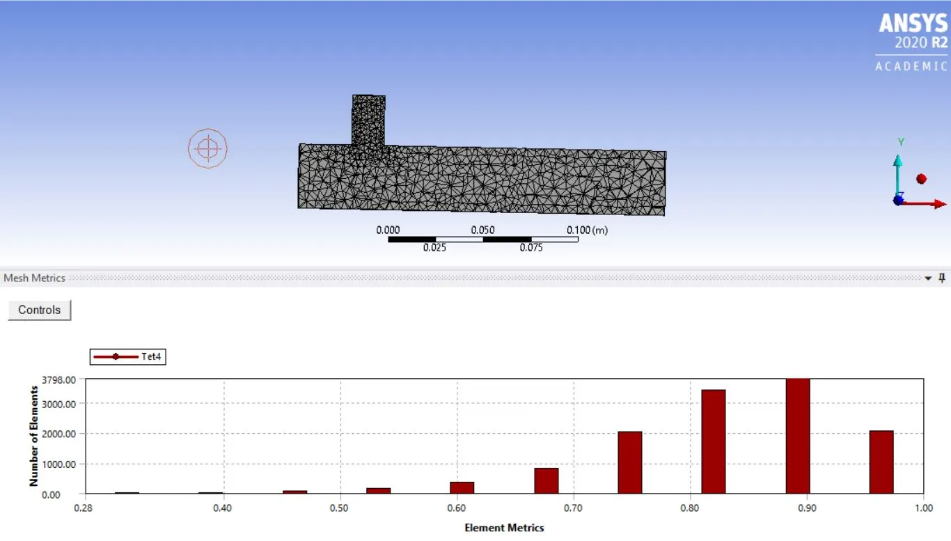
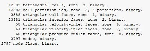
Mesh:

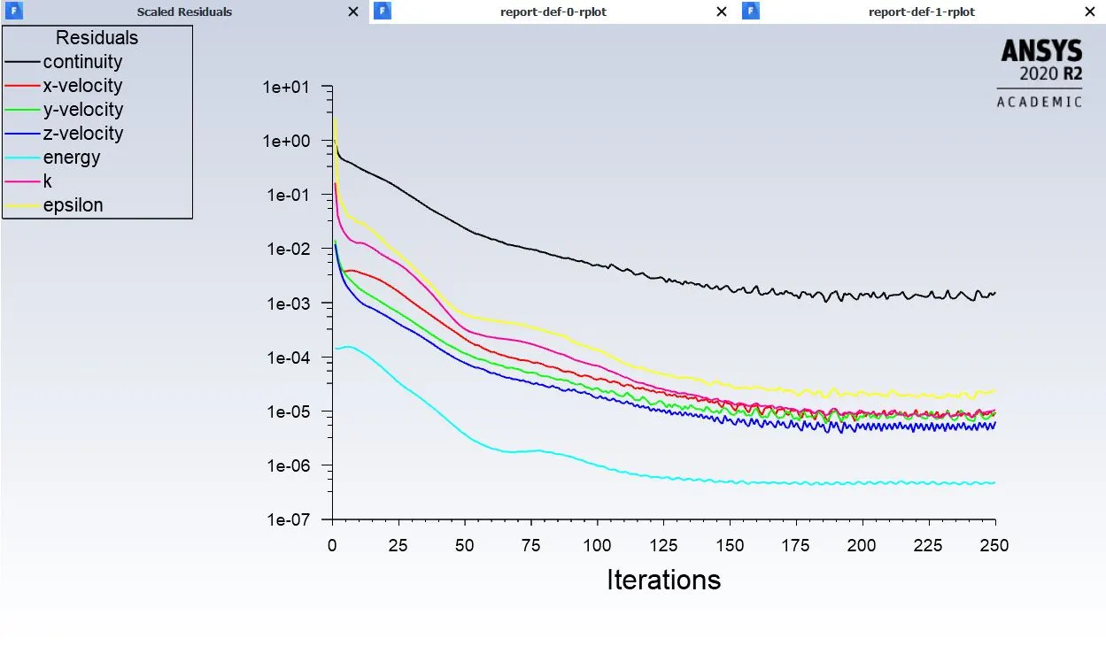
Post processing k epsilon MR 2:

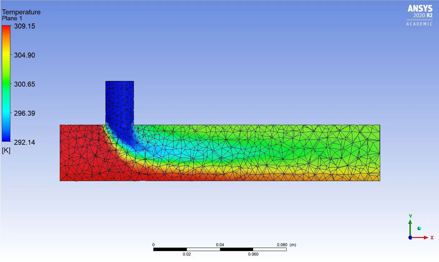
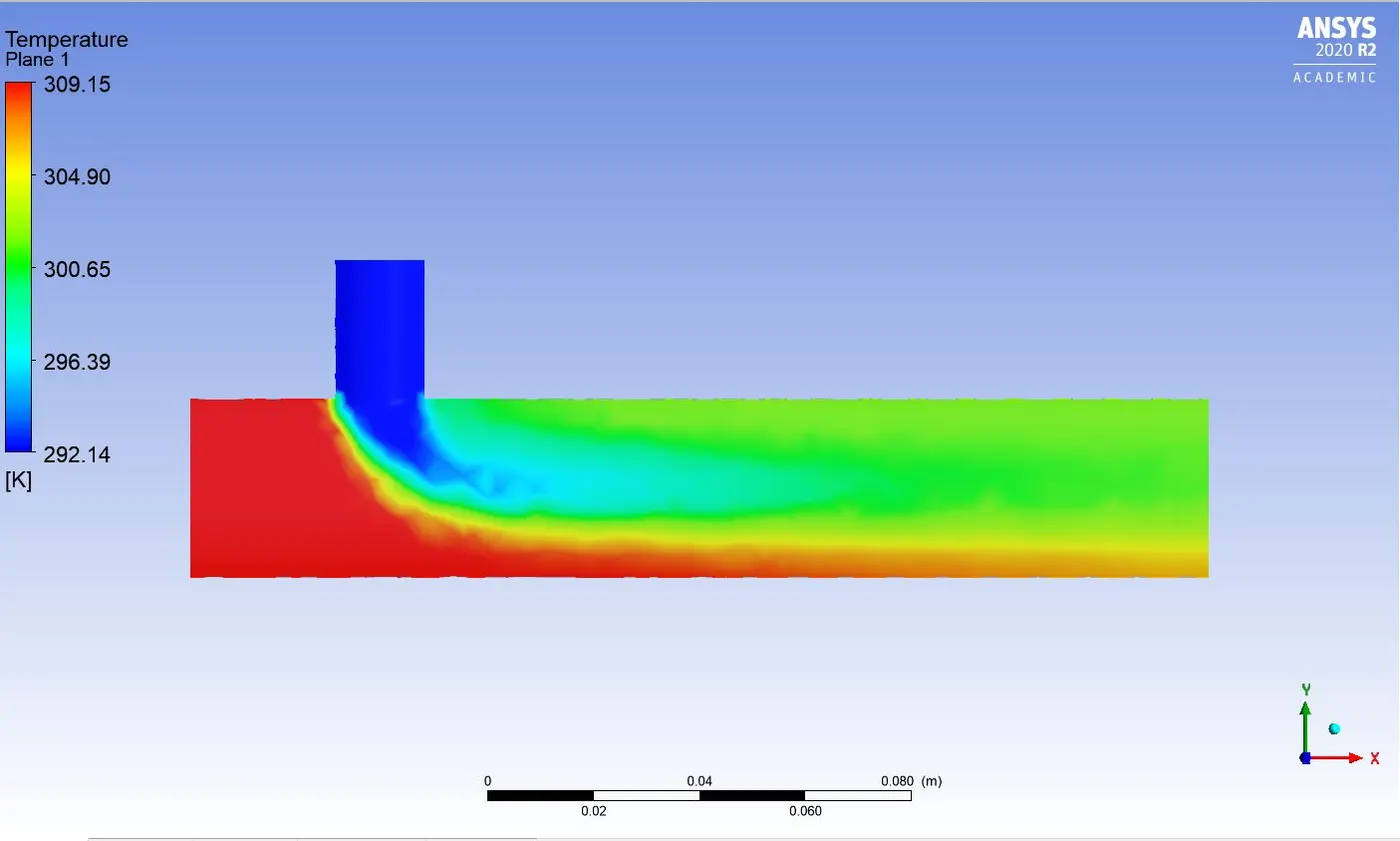
Temperature contour k epsilon MR 2:

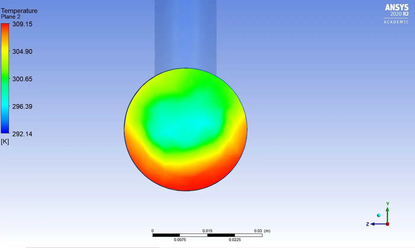
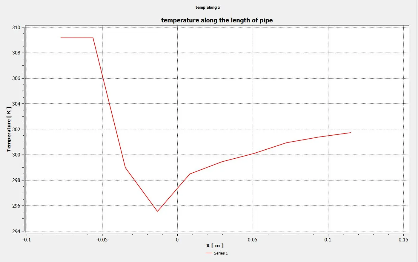
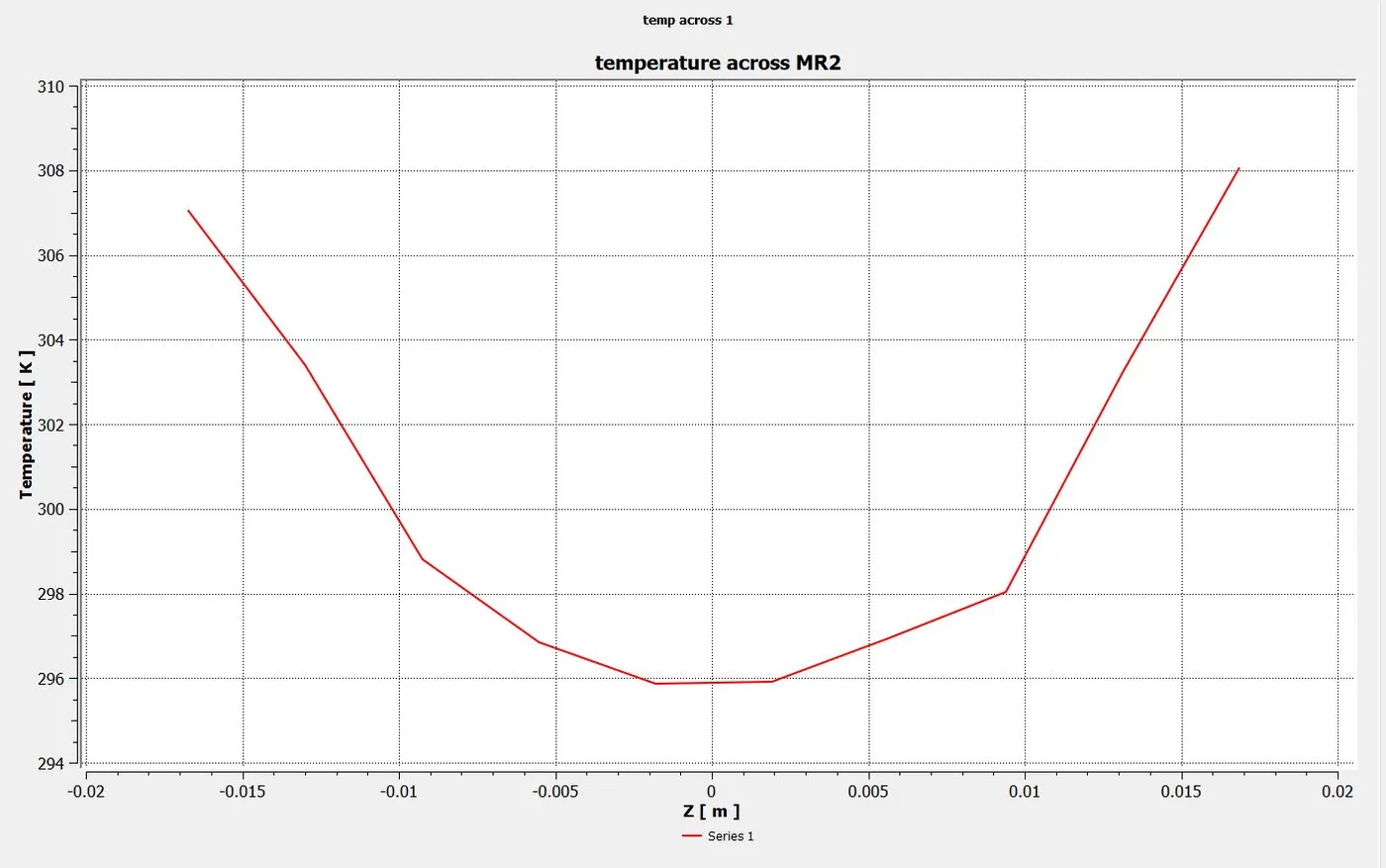
Temperature plot MR_2 k epsilon model along the length of pipe: Temperature plot MR_2 k epsilon model across the length of pipe:

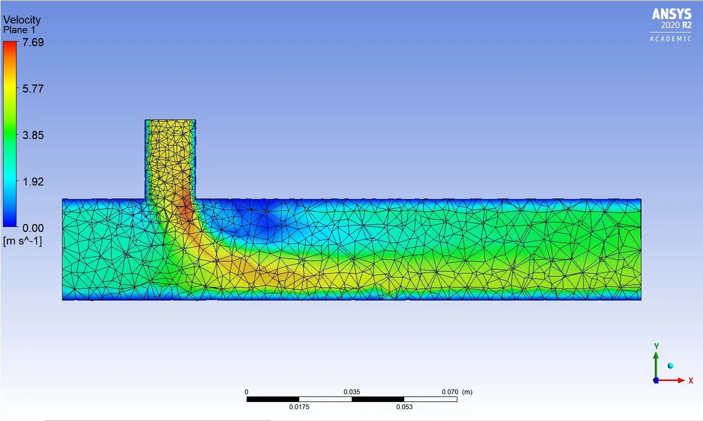
Velocity contour MR_2 for k epsilon model:

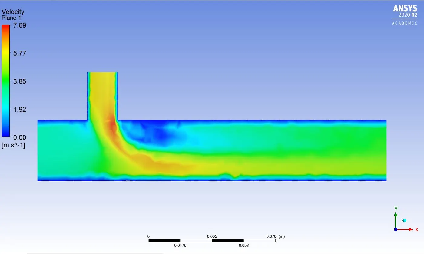
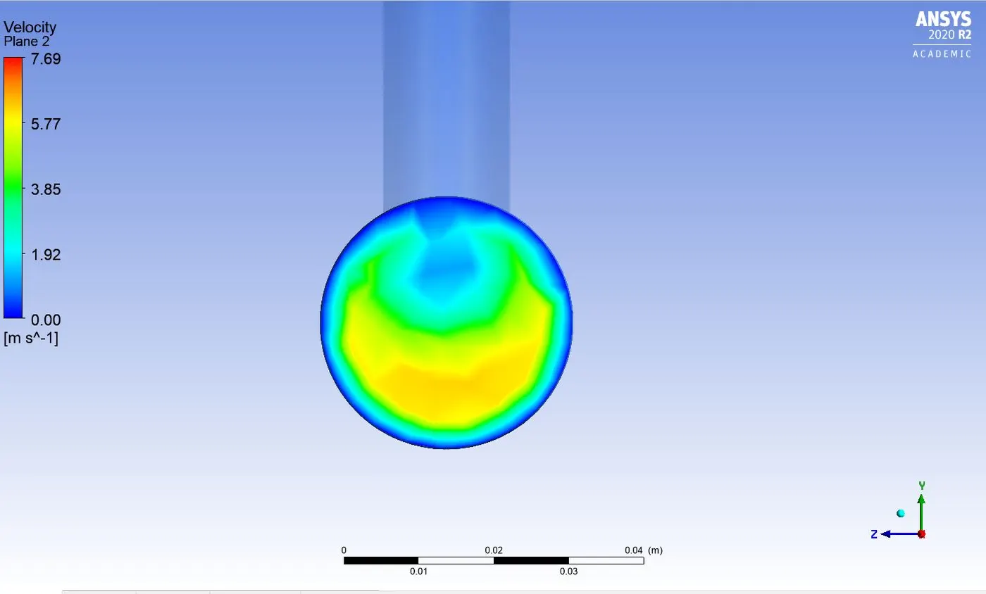
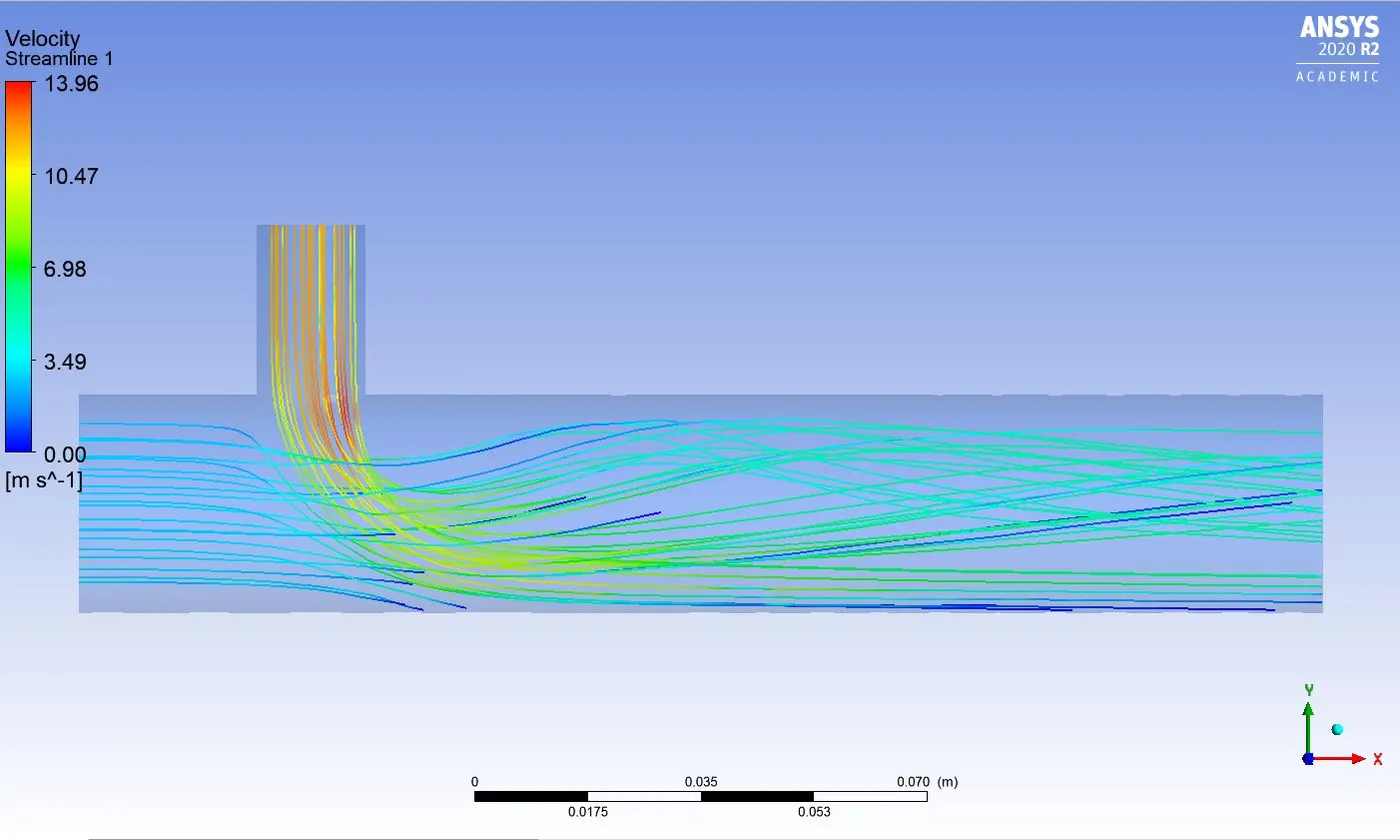
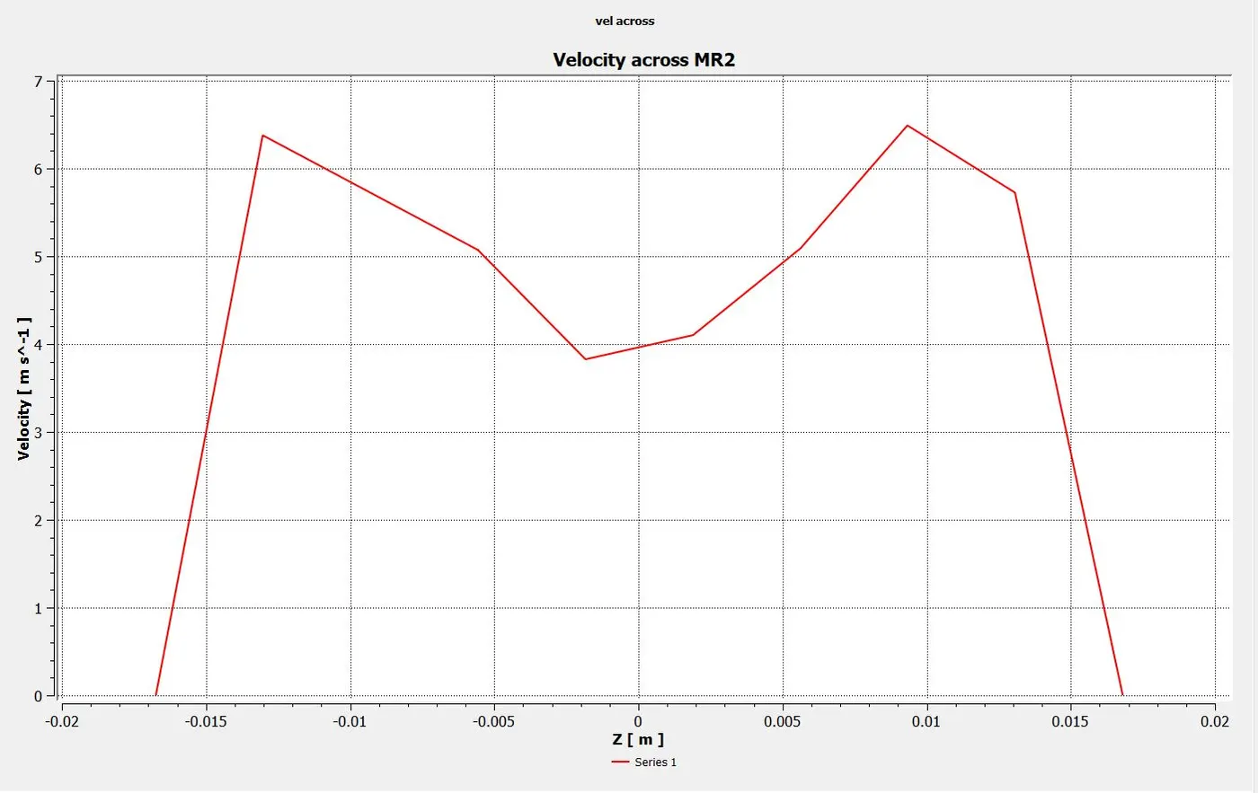
Velocity plot for k epsilon MR_2 along the length of pipe: Velocity plot for k epsilon MR_2 ACROSS the length of pipe:

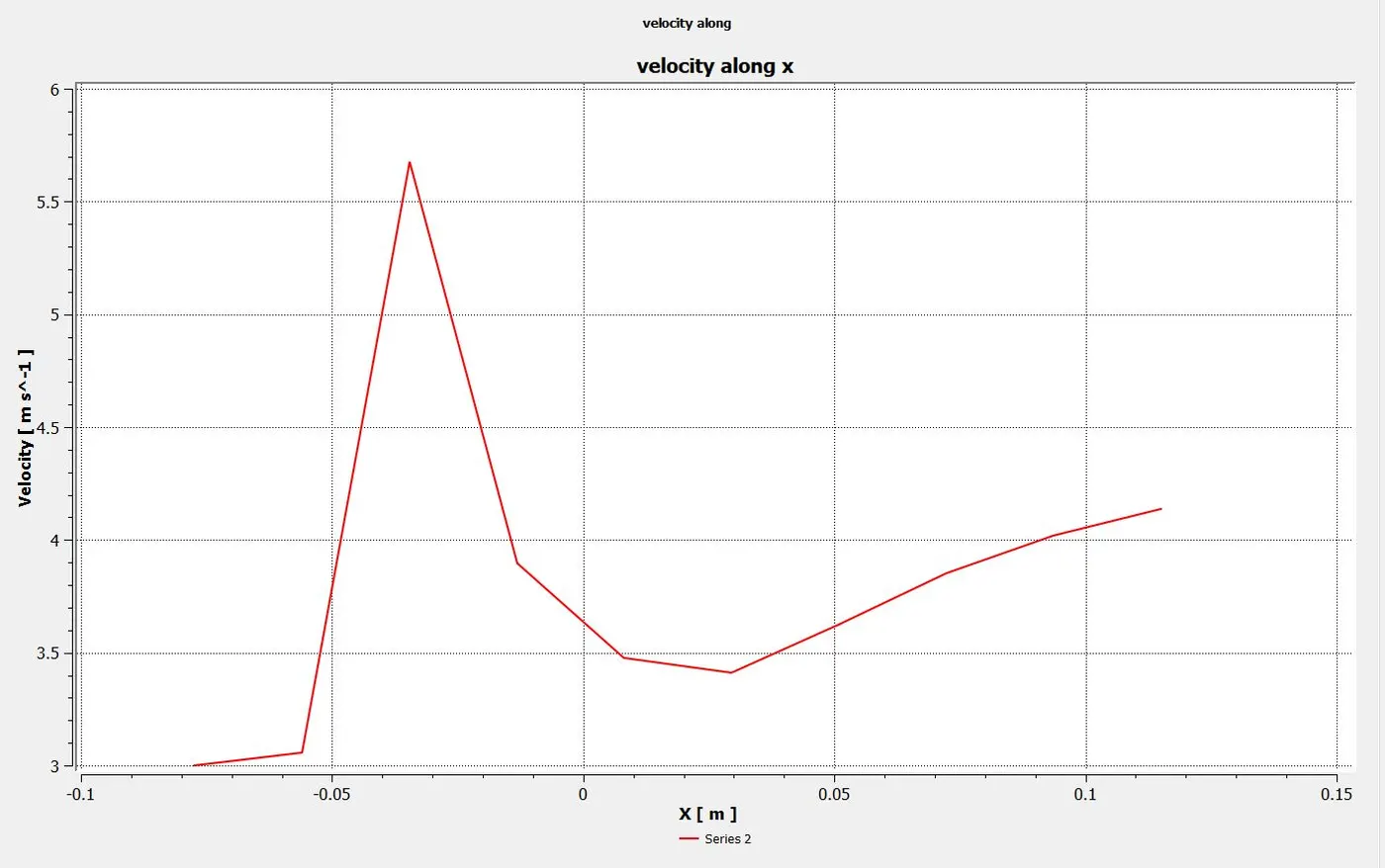
Case 1:

k epsilon model with MR=4

Post processing k epsilon MR 4:

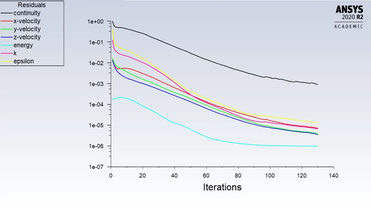
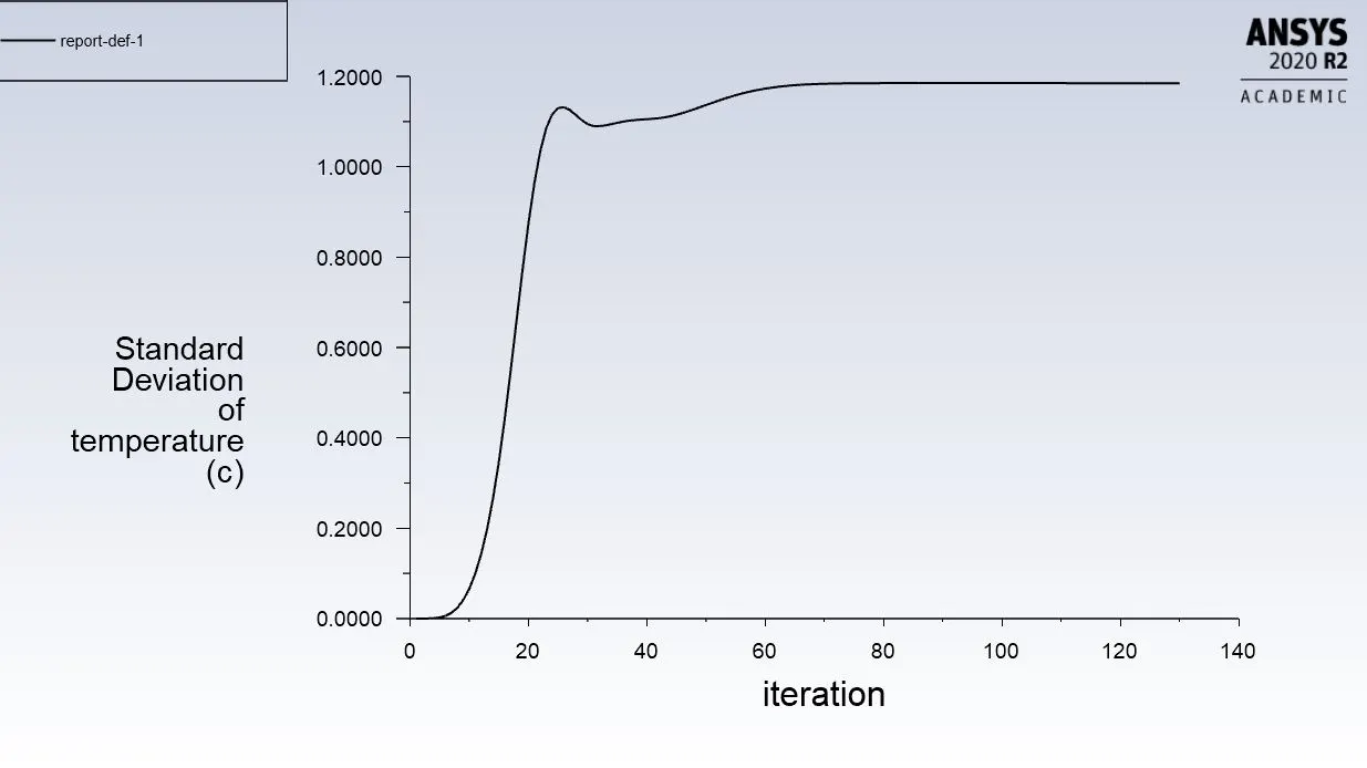
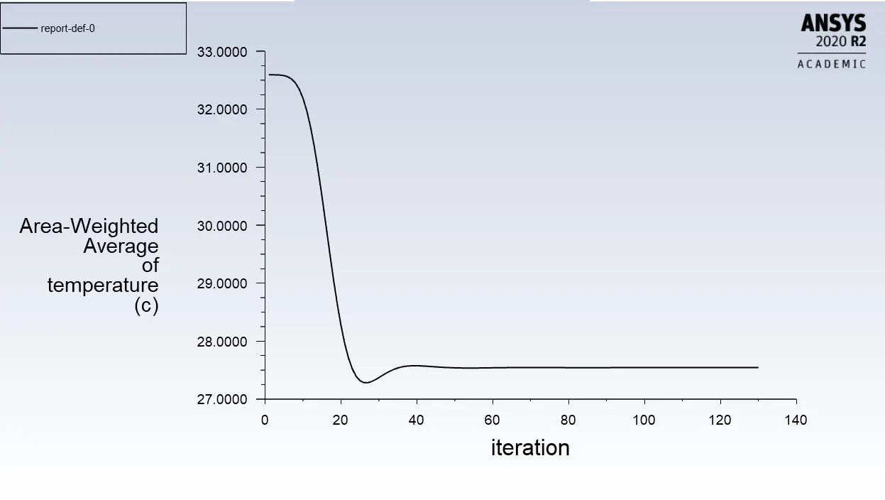
Temperature contour k epsilon MR 4:

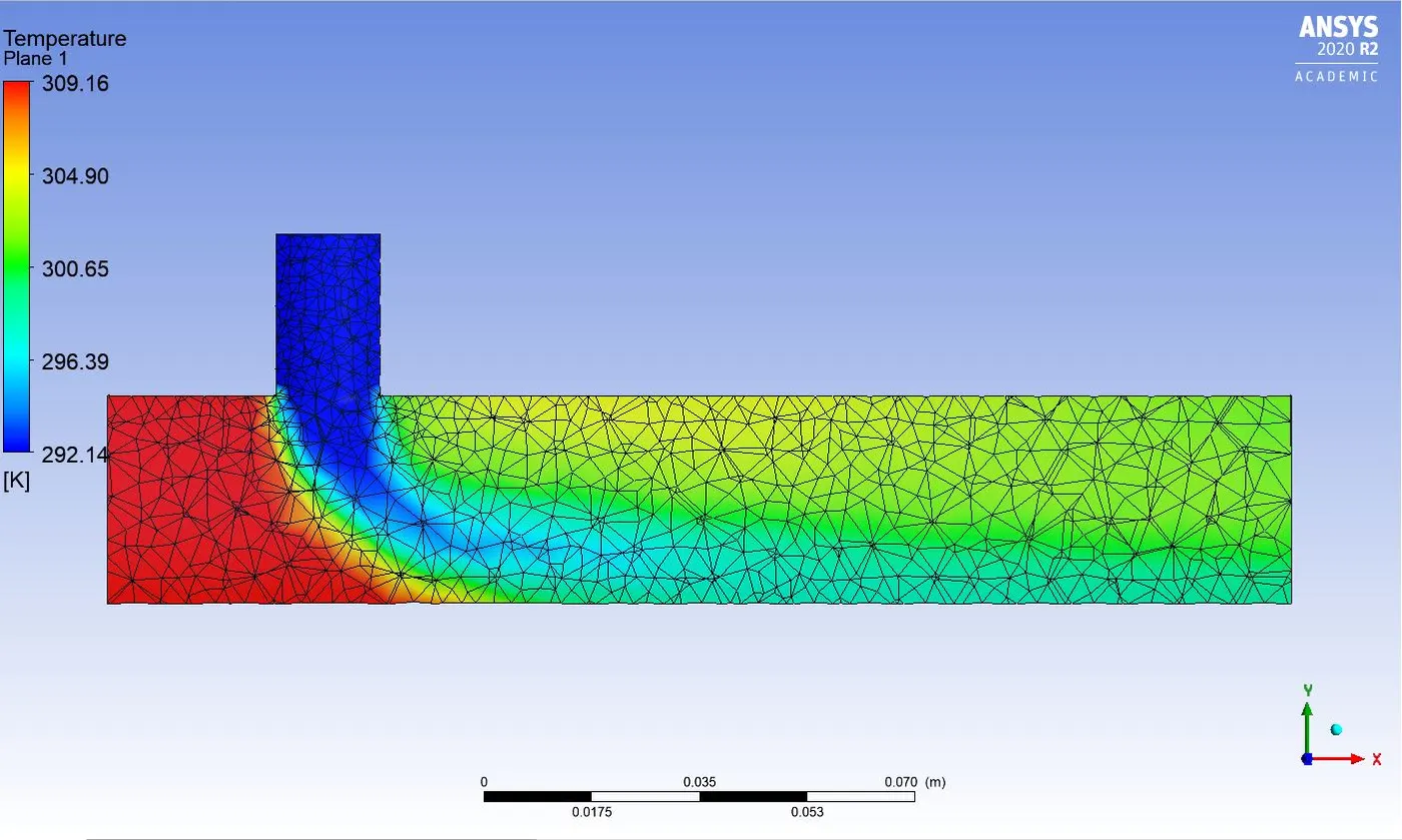
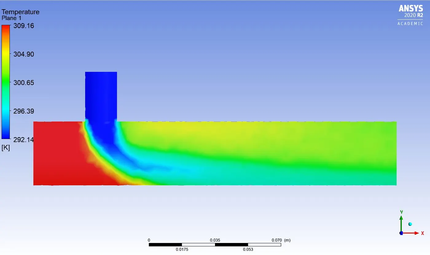
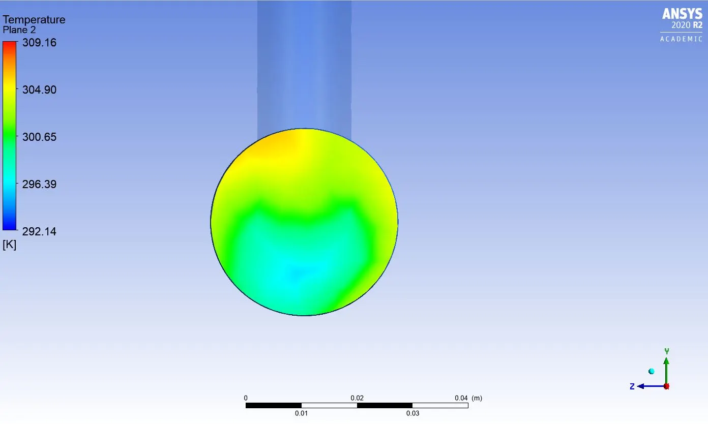
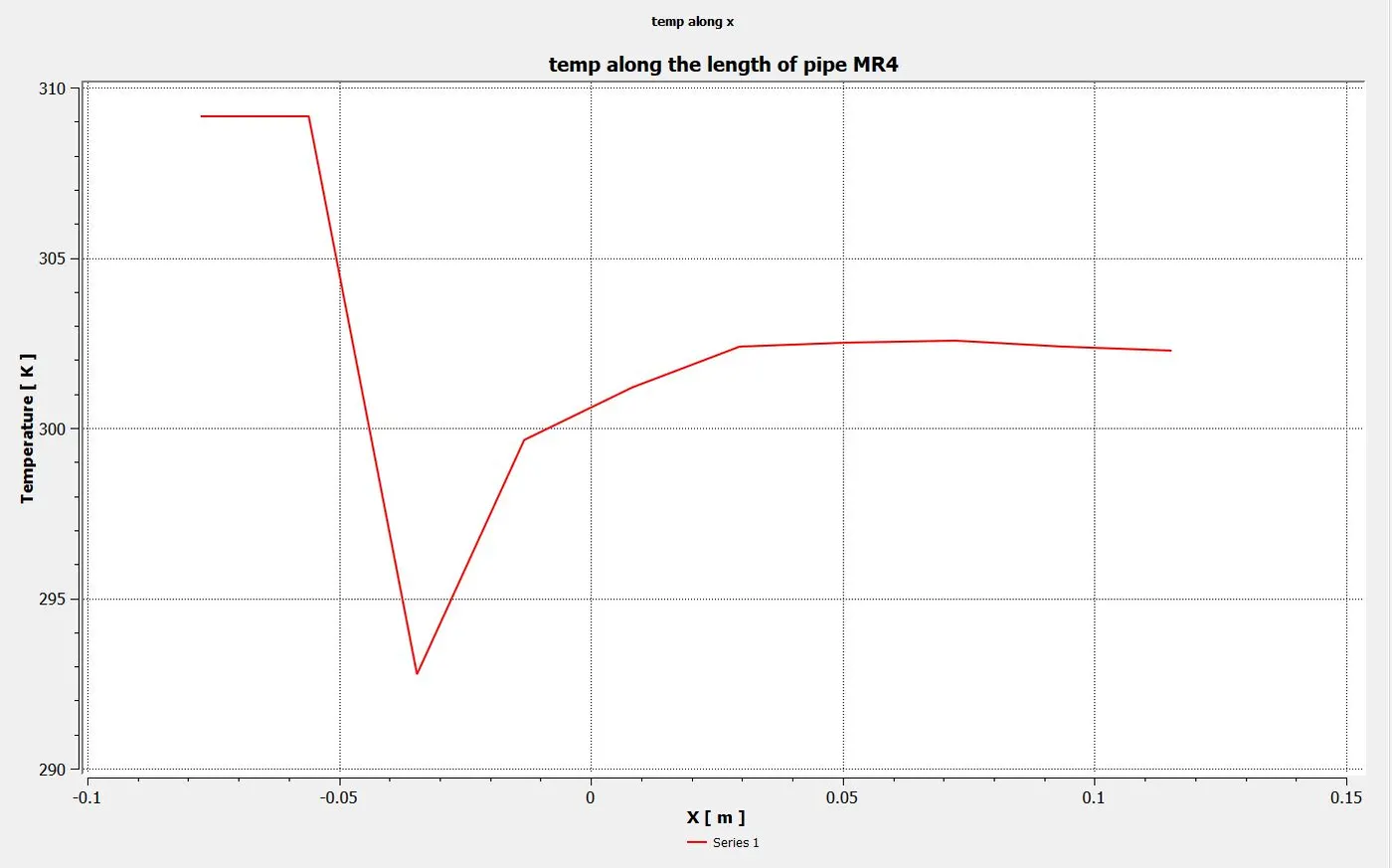
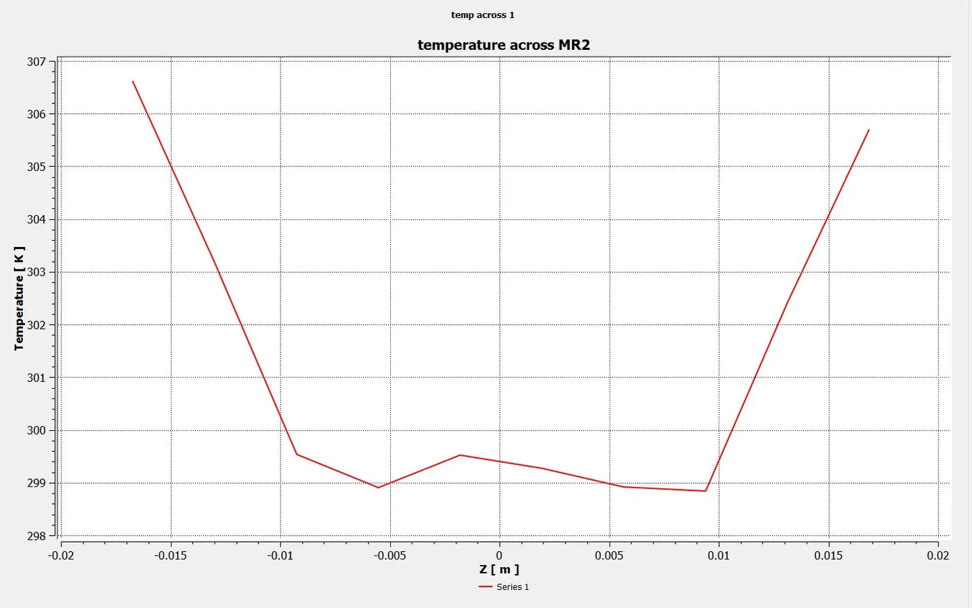
Temperature plot for k epsilon model MR 4 along the length of pipe: Temperature plot for k epsilon model MR 4 across the length of pipe:

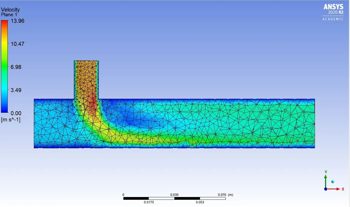
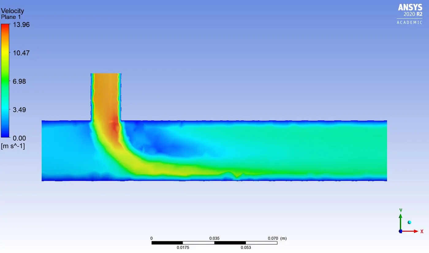
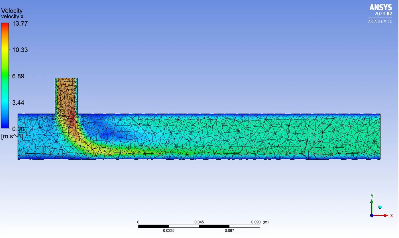
velocity contour k epsilon MR 4:

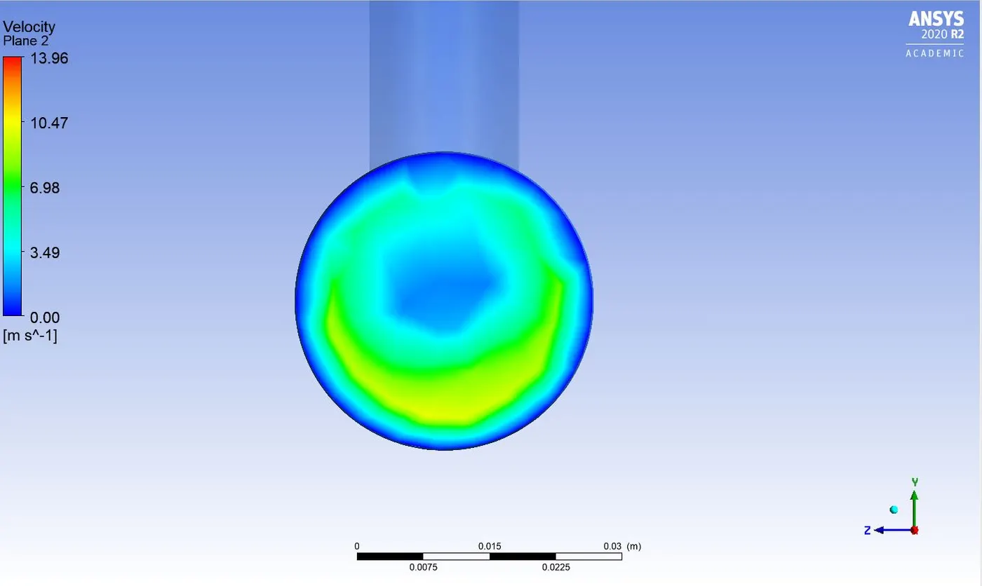
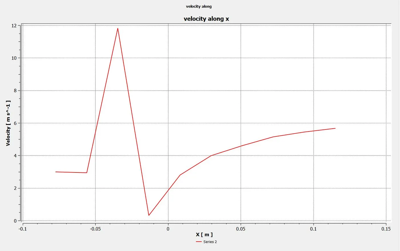
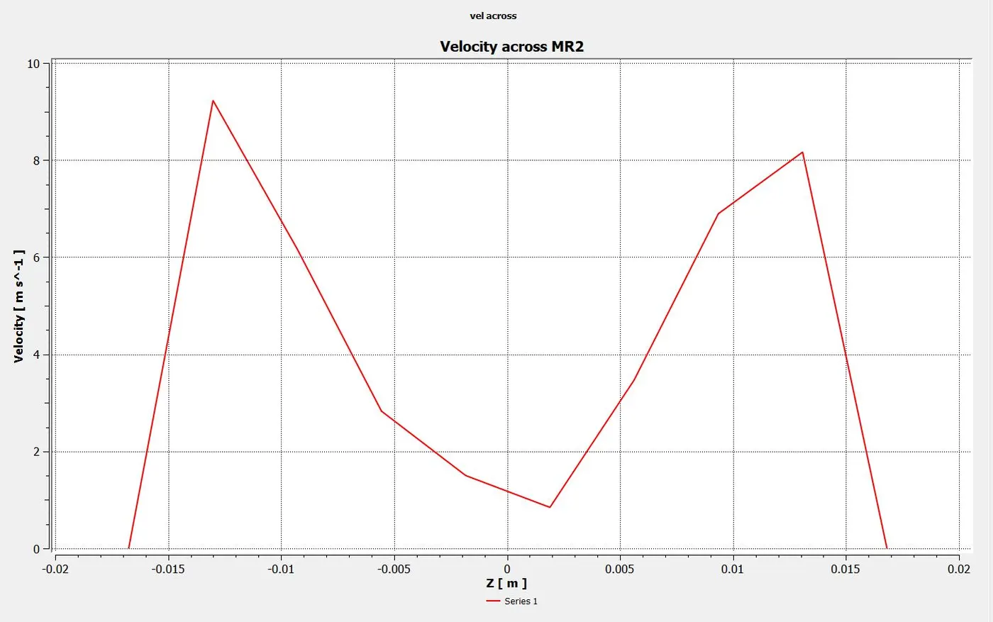
velocity plot k epsilon MR 4 along the length of pipe: velocity plot k epsilon MR 4 across the length of pipe:

K-omega model

K-omega model

Now by using K-omega model for case 1 short tee:

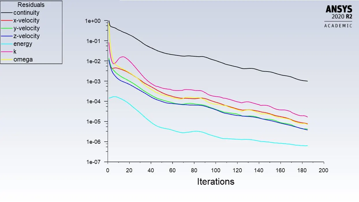
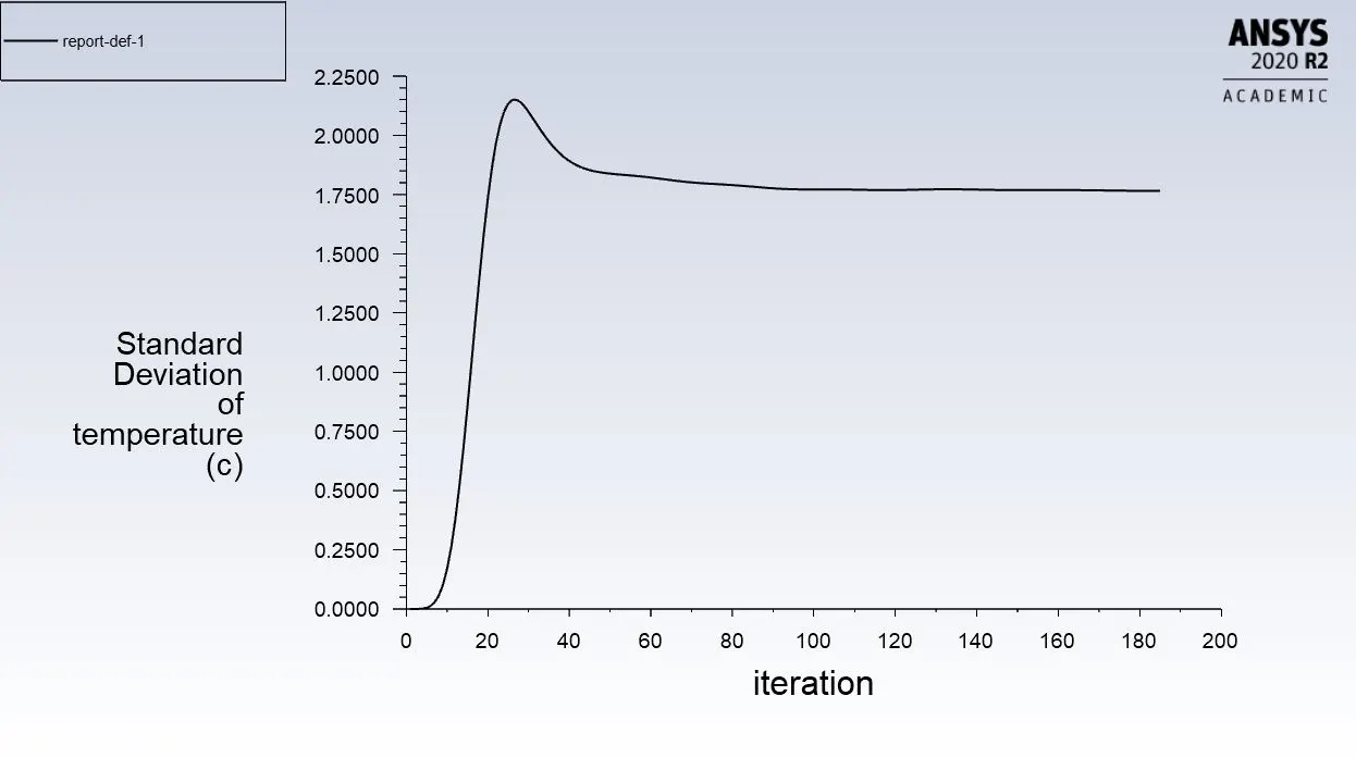
Post processing case 1 k-Omega MR 2:

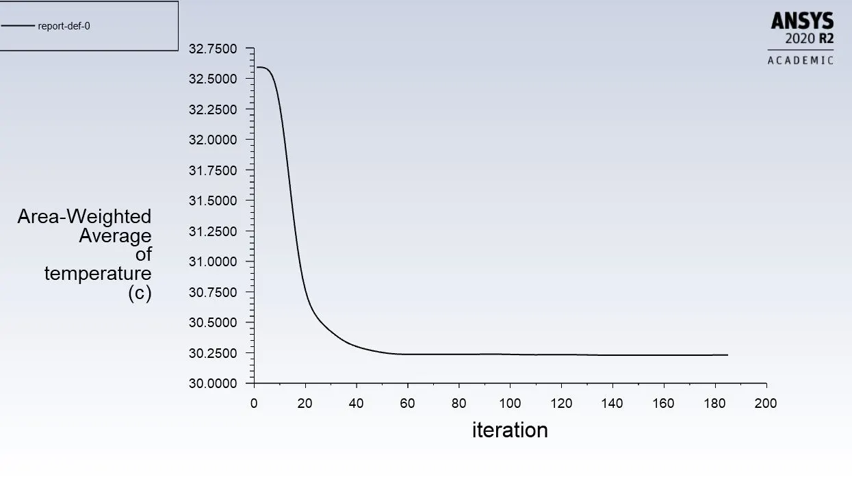
Temperature contour k omega MR 2:

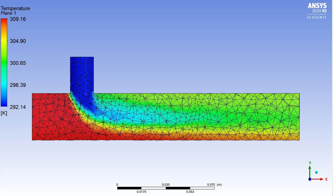
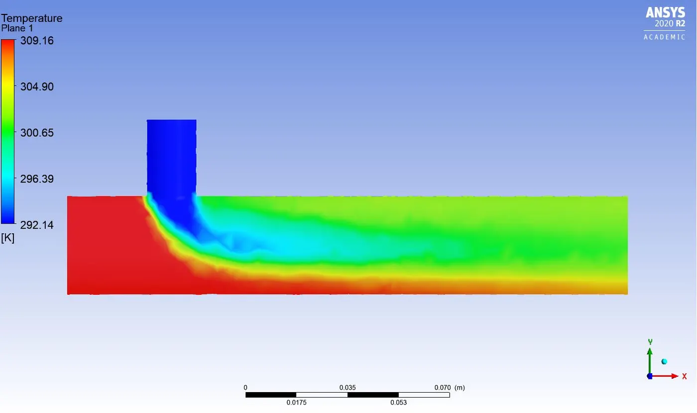
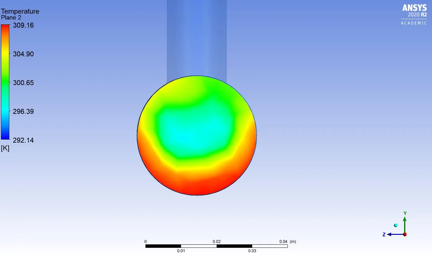
Temperature plot k omega MR 2 along the length of pipe: Temperature plot k omega MR 2 across the length of pipe:

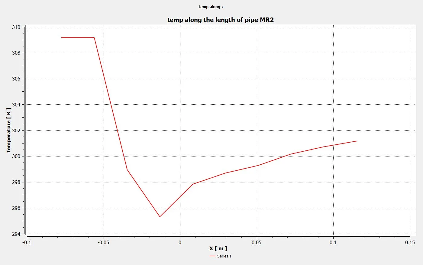
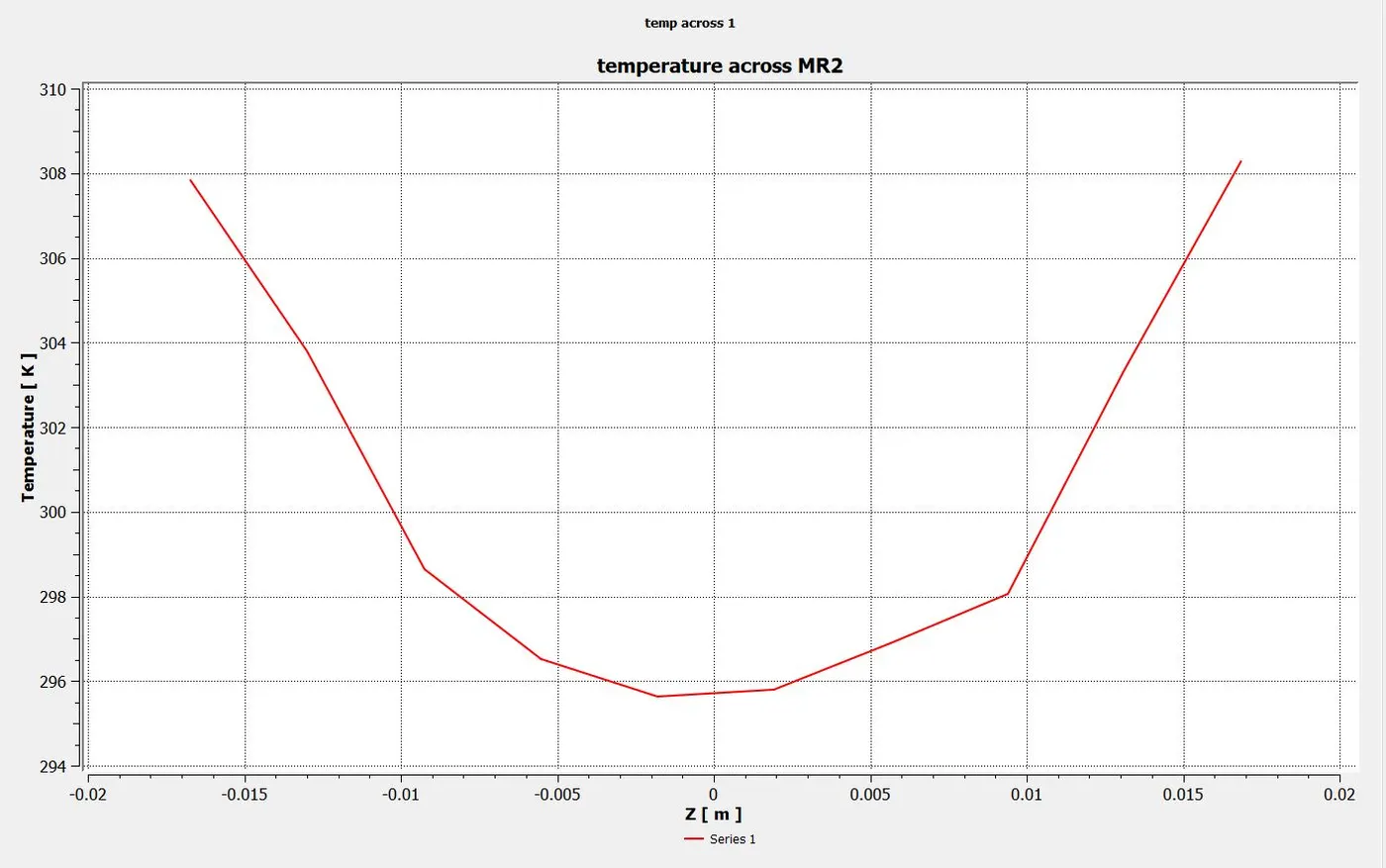
velocity contour k omega MR 2:

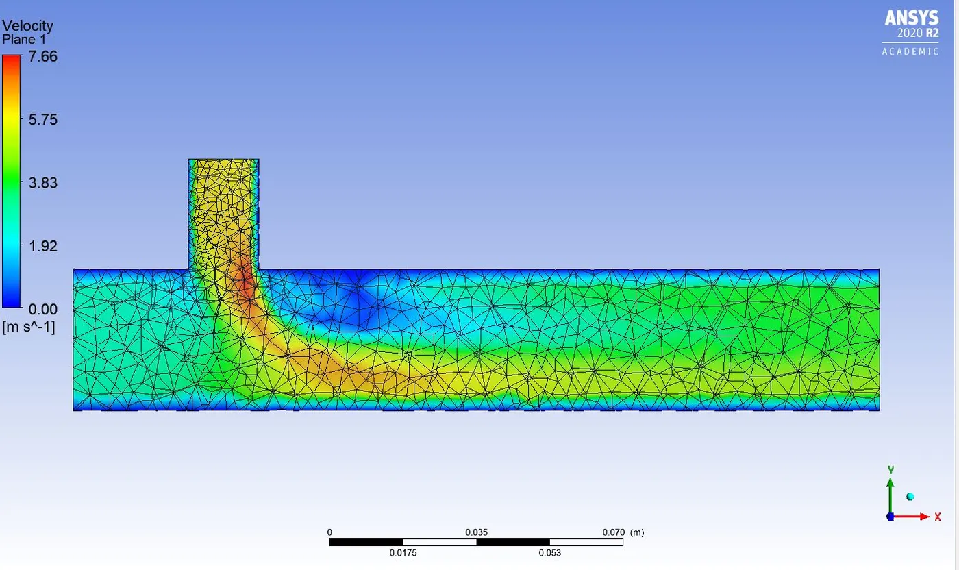
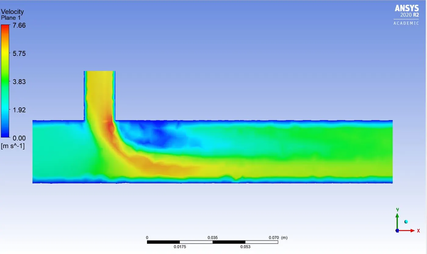
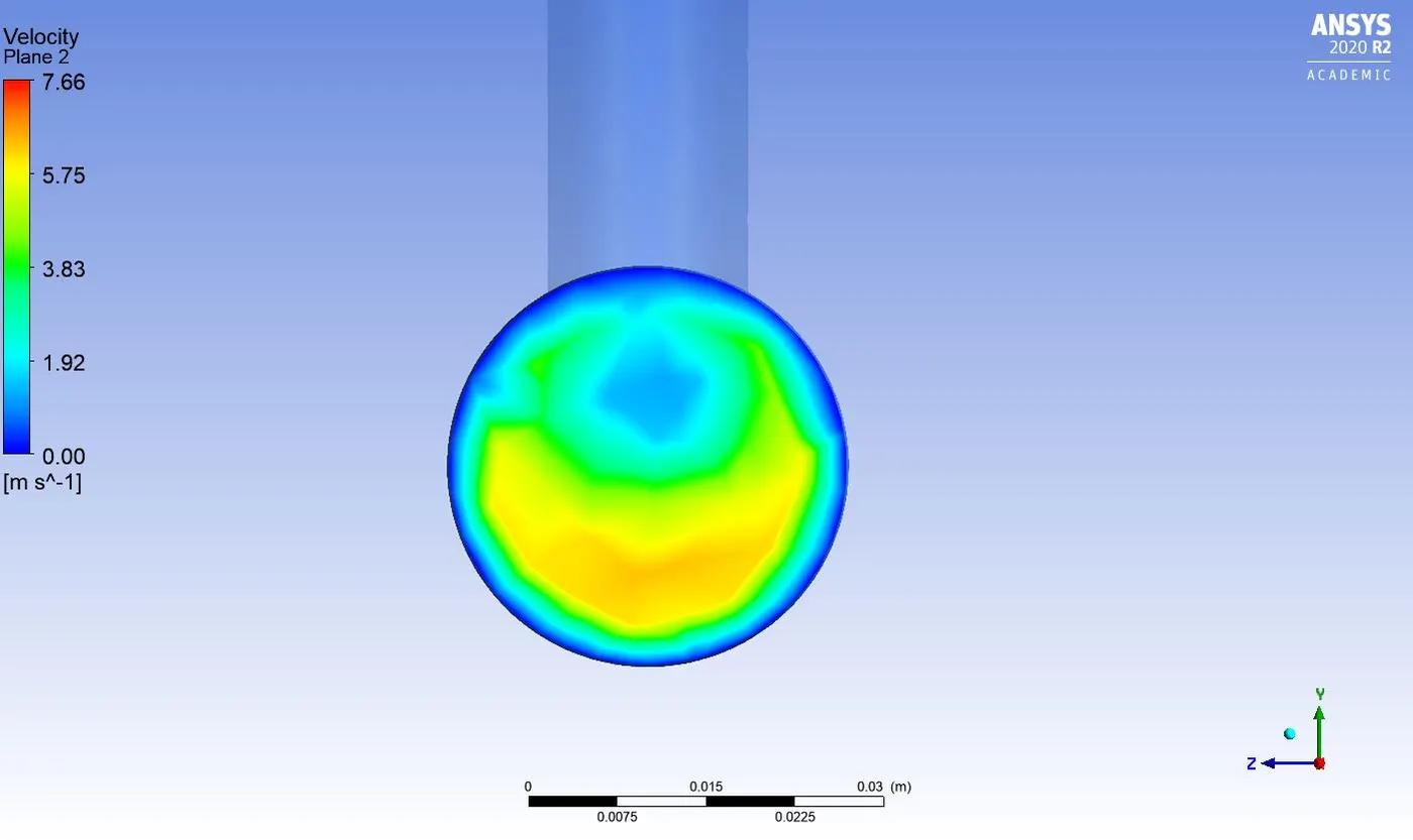
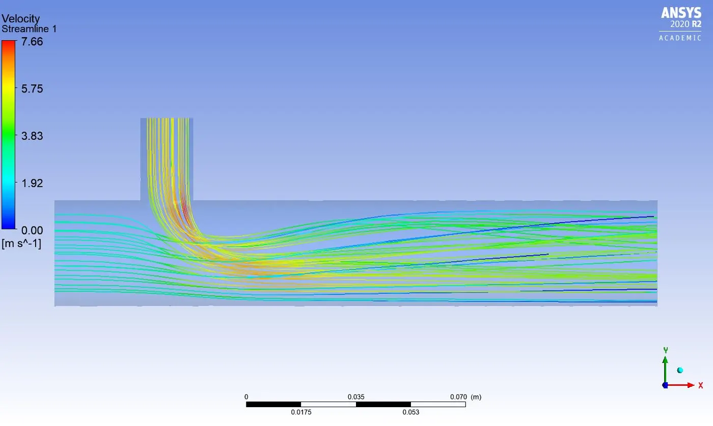
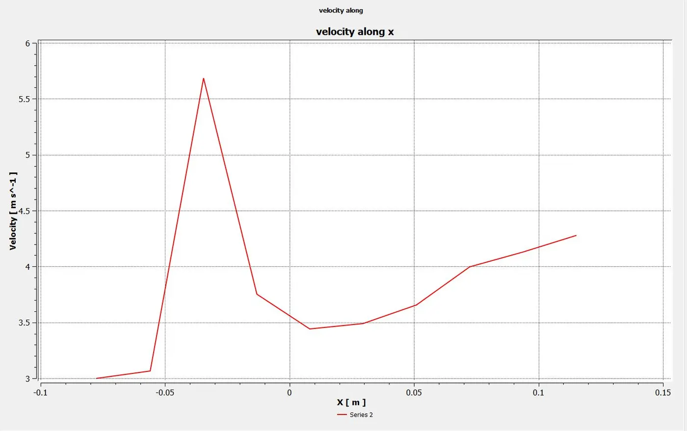
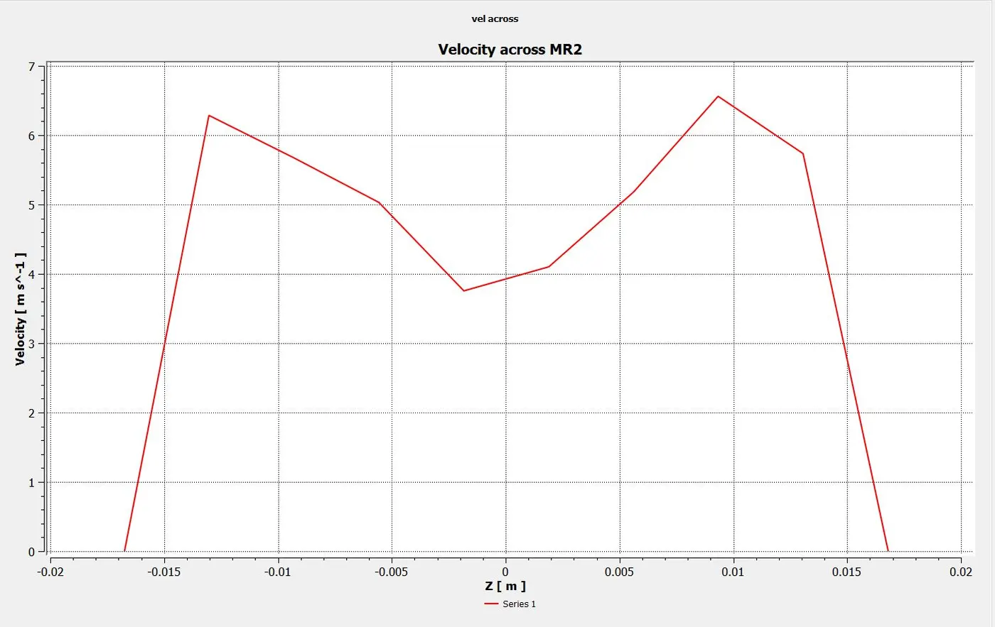
Velocity plot k omega MR 2 along the length of pipe: velocity plot k omega across length of pipe

case 1 k short tee k omega MR 4:

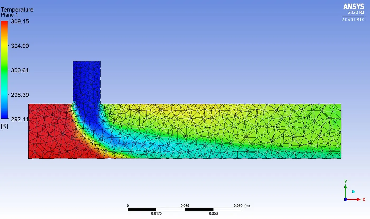
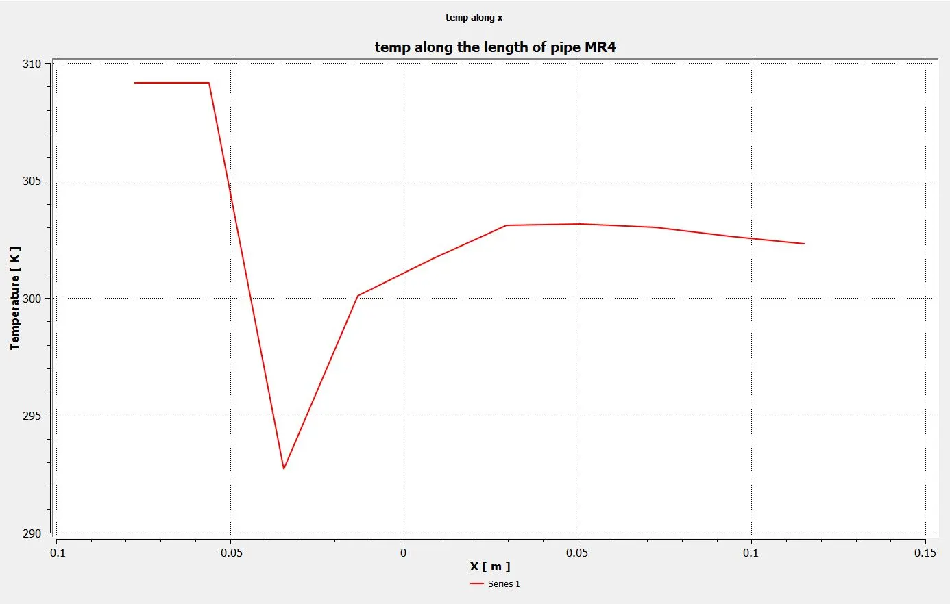
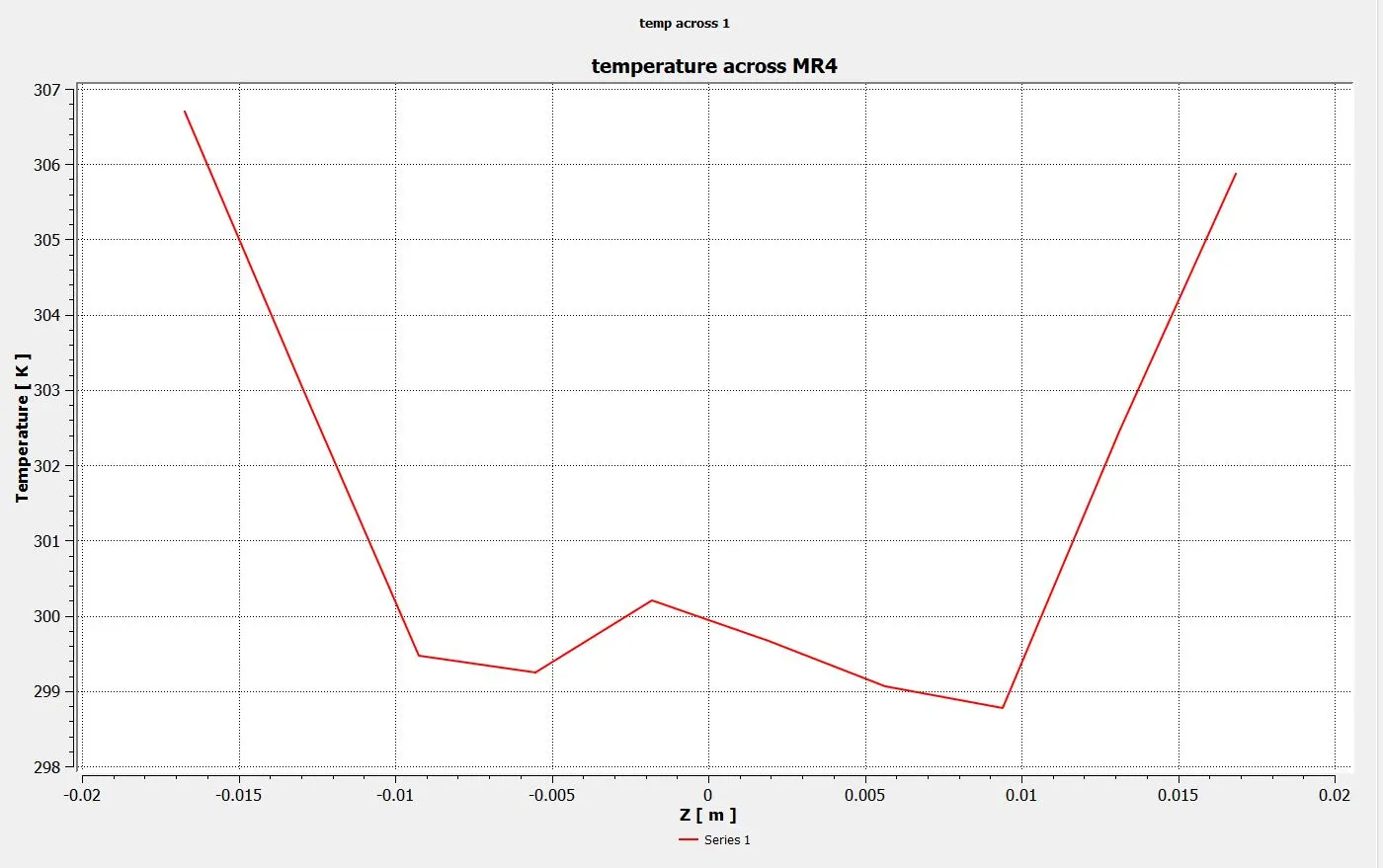
Post processing case 1 k-Omega MR 4:

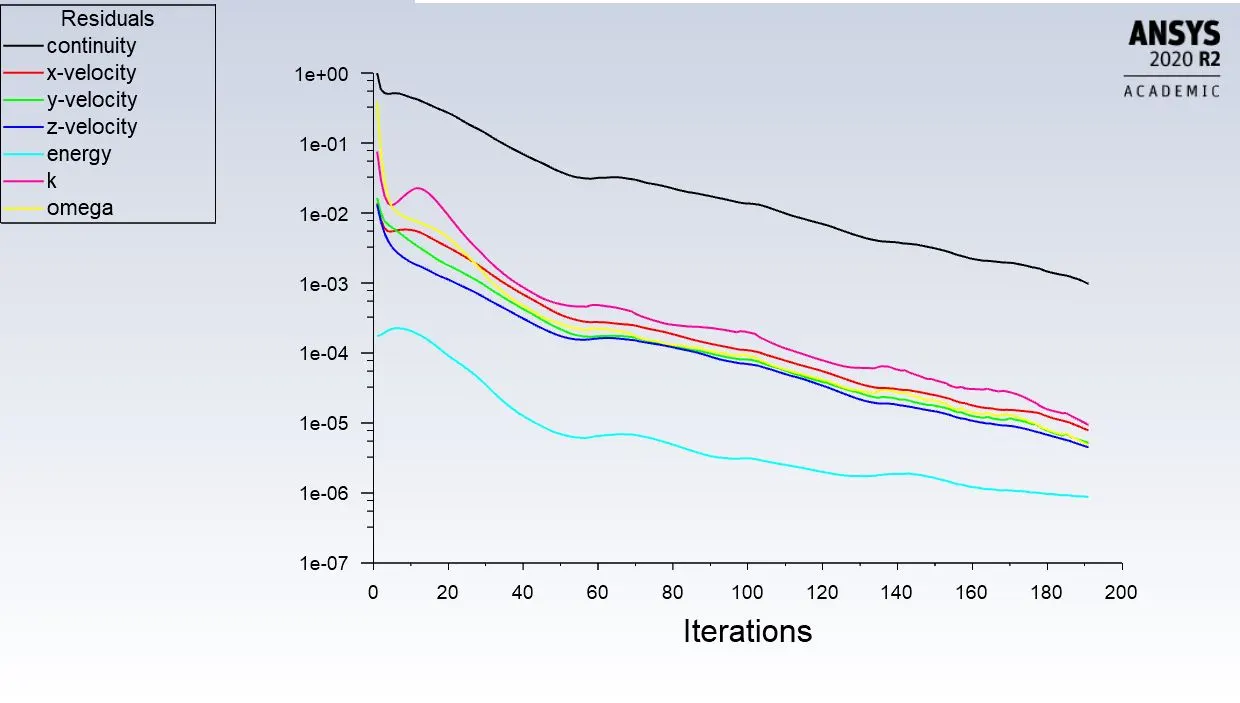
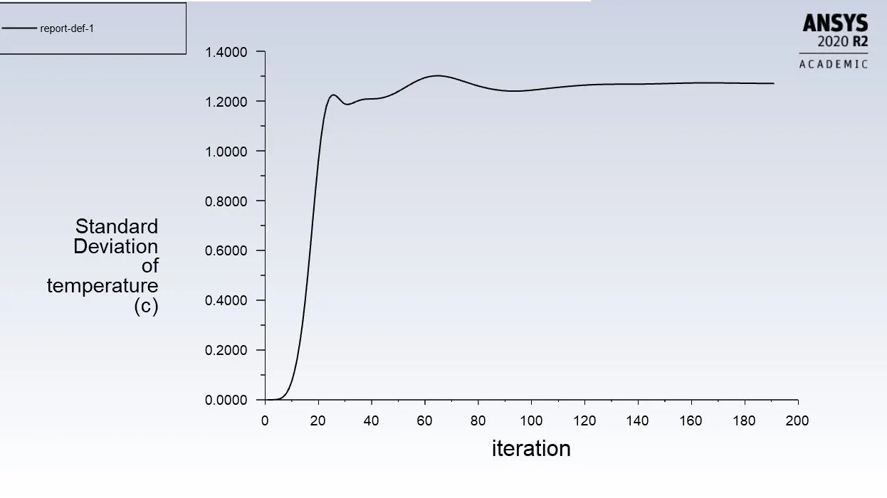
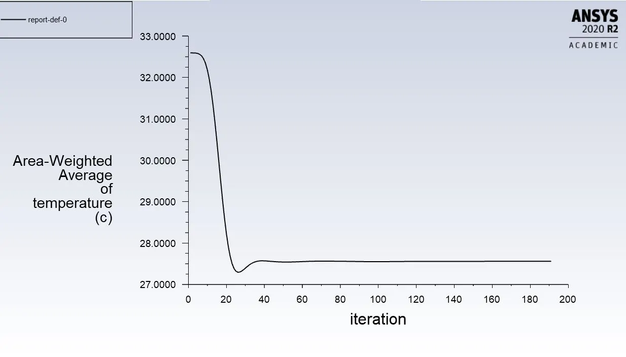
Temperature contour k omega MR 4:

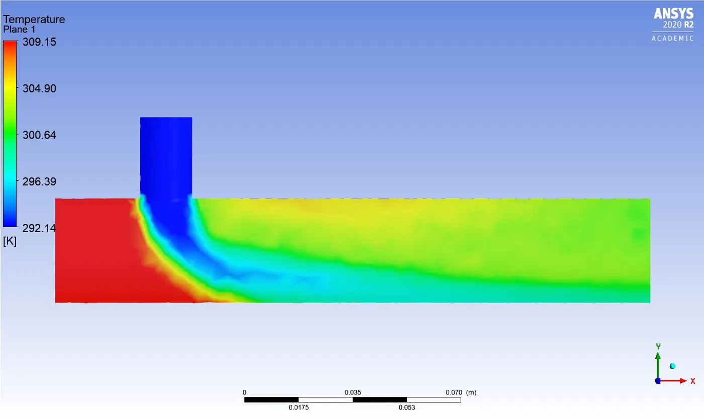
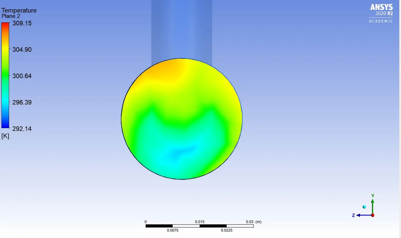
Temperature plot k omega MR 4 along the length of pipe: Temperature plot k omega MR 4 across the length of pipe:

Velocity contour k omega MR 4:

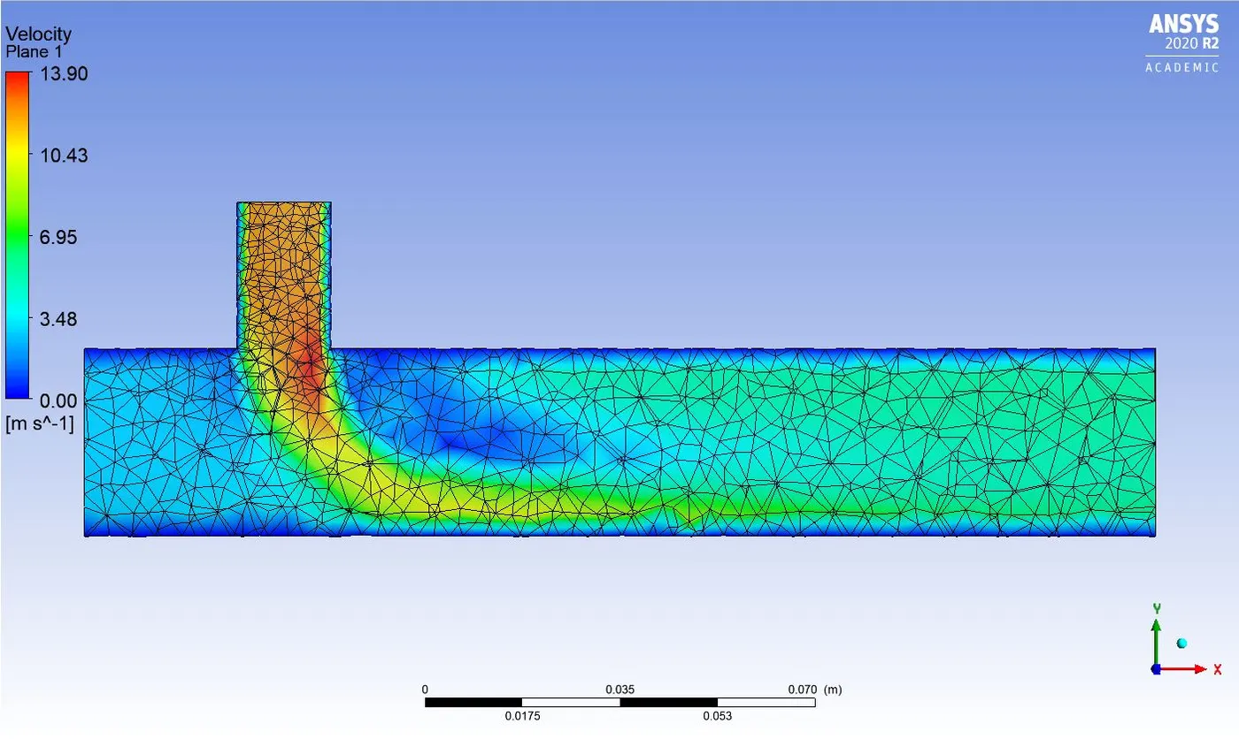
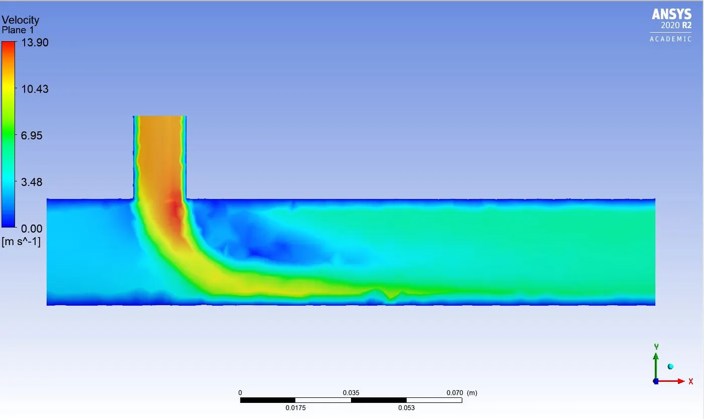
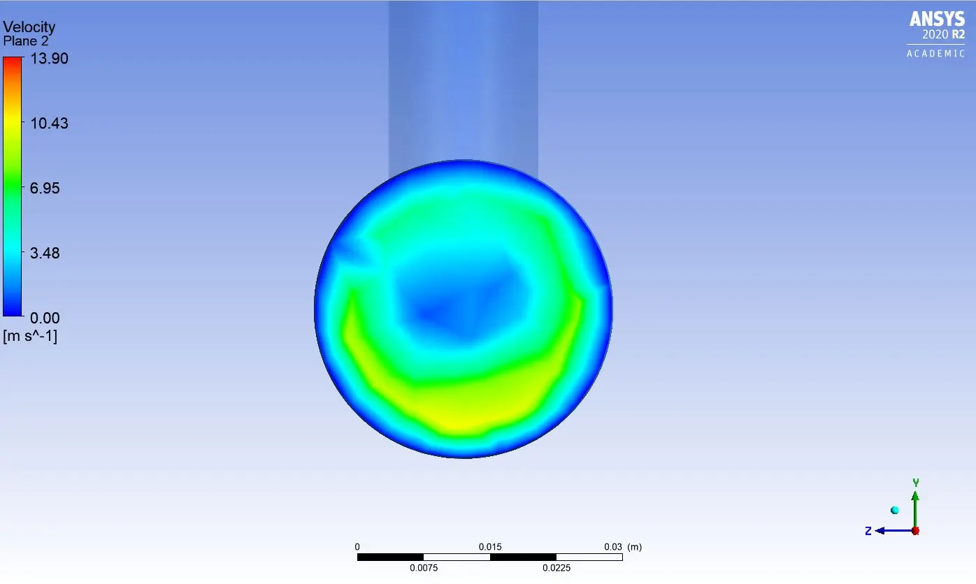
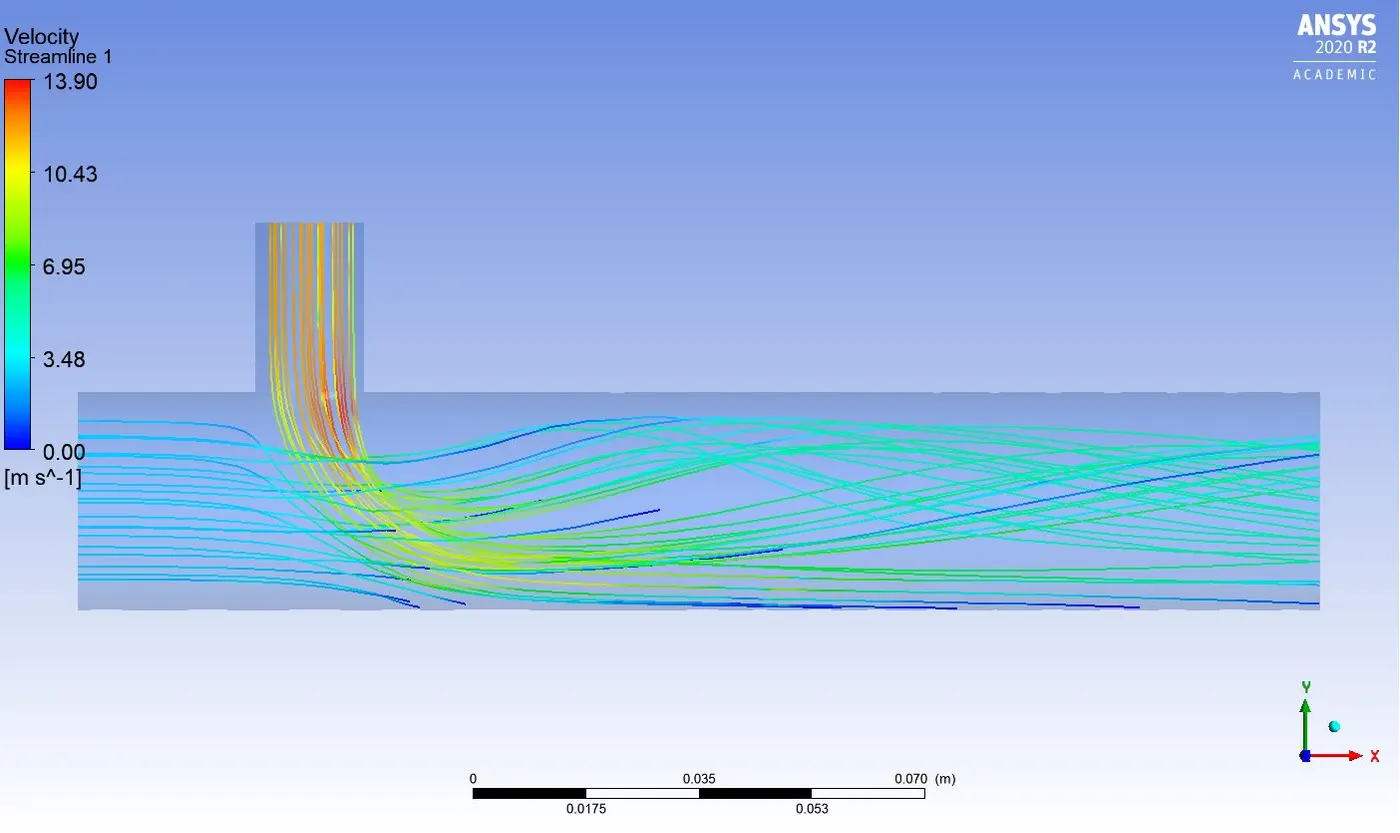
Velocity plot k omega MR 4 along the length of pipe: Velocity plot k omega MR 4 across the length of pipe:

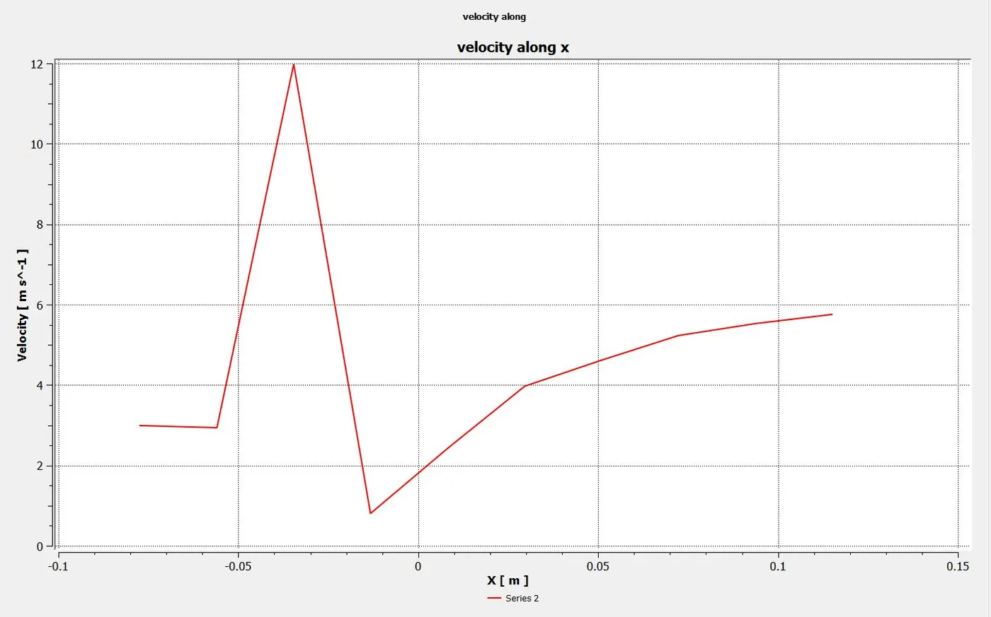
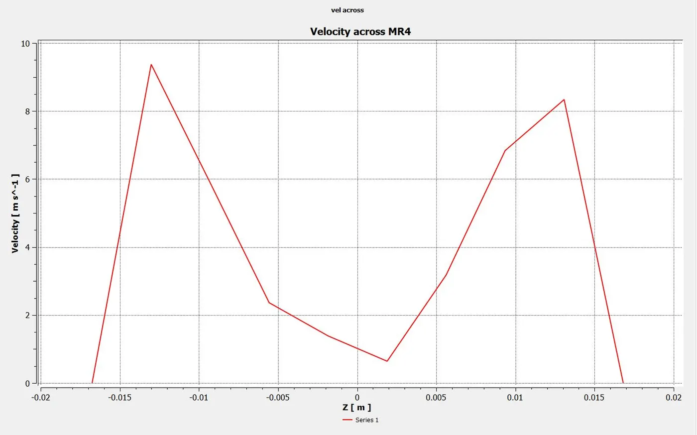
Table of k epsilon and k-omega sst turbulence model for short tee

------------>>Now we need to calculate the analytical solution inorder to compare with the average temperature we got by simulation to check for accuracy and to proceed with better model for case 2 which is the long tee model.

Analytical solution:

Formula for Tmix:

The fluid under analysis is air which has density of 1.225kg/m^3

Temp at inlet x (hot fluid)= 36 degrees

Temp at inlet y (cold fluid)= 19 degrees

For Momentum ratio 2:

mass flow rate x= 0.0033 kg/s

mass flow rate y= 0.0016 kg/s

Tmix=30.45 degrees celsius

For Momentum ratio 4:

mass flow rate x= 0.0033 kg/s

mass flow rate y= 0.0033 kg/s

Tmix=27.5 degrees celsius

Conclusions to be made according to the above data :

• Both turbulence models gives almost same results.
• Standard deviation of k-epsilon model is less than k-omega model by a small amount.
• In this we can say that k-epsilon is a better model due to less standard deviation which means more accuracy in calculations
• Generally speaking about turbulence models k- epsilon is used where flow does not demand to integrate the solution through the viscous layer and wall boundaries are secondary which briefly do not take into account the laminar sublayer. The calculation starts from a certain y+ distance from wall.
• As the k-epsilon is a high reynolds number model the k epsilon is better suited for this procedure by which the convergence of solution is faster.
• k-omega is used for near wall simulation to gather the effect of viscous sublayer and as it has high standard deviation and high residual errors than k-epsilon ,so k-epsilon is preferred

So now we go on by k-epsilon model for case 2.

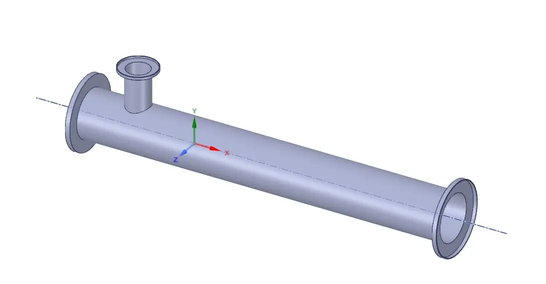
CASE 2: Long tee model

Geometry:

its a long tee model:

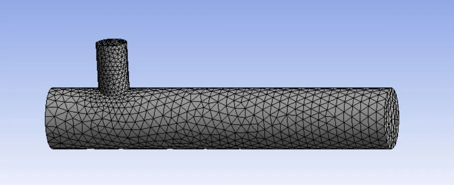
Meshing along with mesh quality:

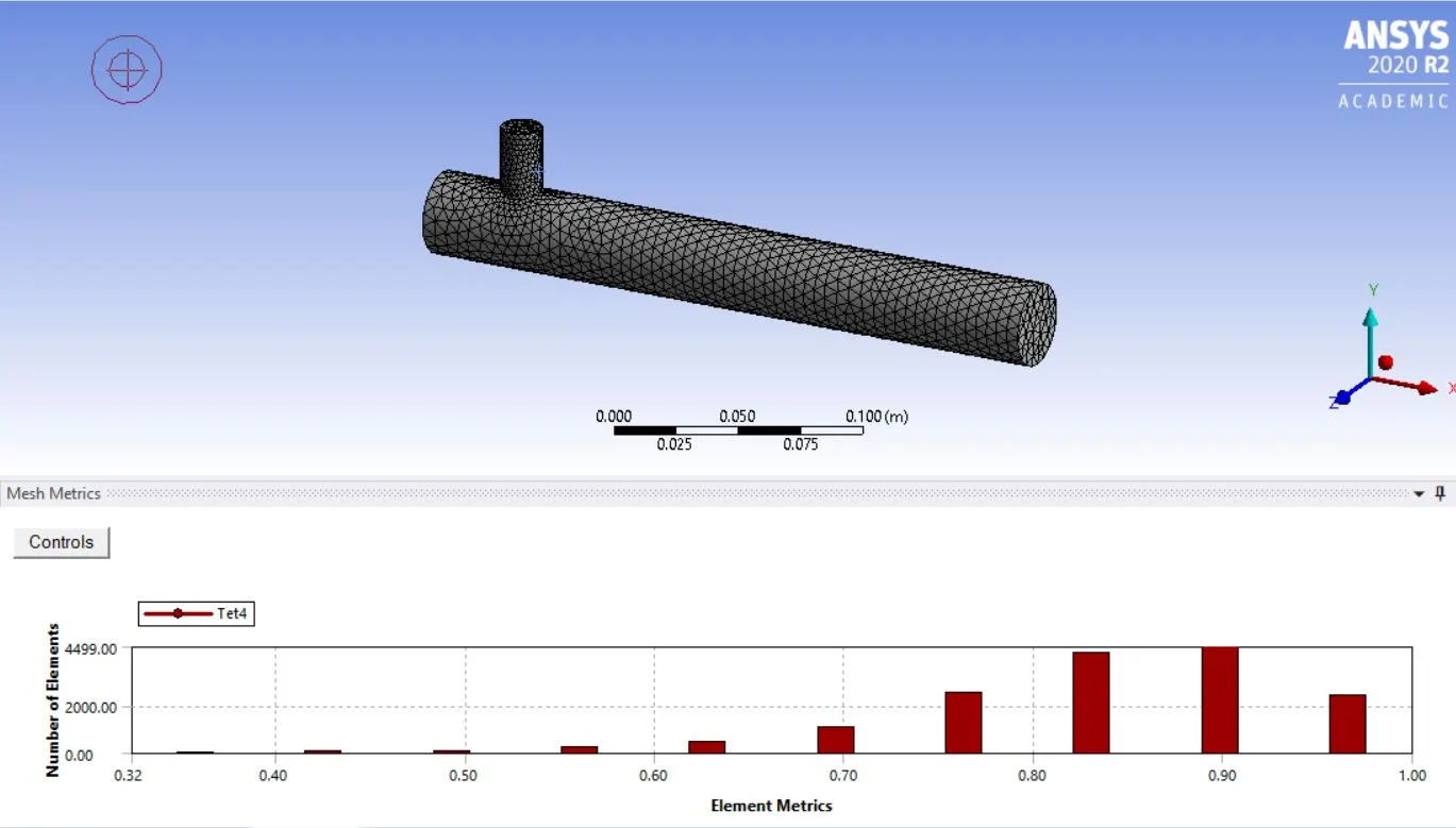
no of elements: 15483(total)

nodes : 3448

size : 2.7mm

Setup:

k epsilon model is taken into account with realizable model.

Boundary condition:

Momentum ratio 2:

Velocity inlet x=3m/s

velocity inlet y=6m/s

inlet temp x=36 degrees celsius

inlet temp y= 19 degrees celsius

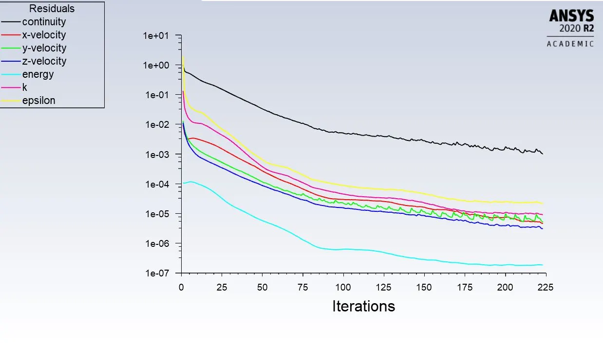
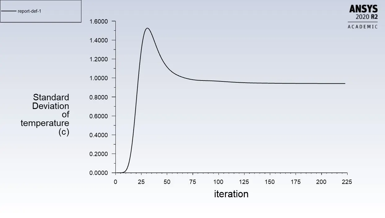
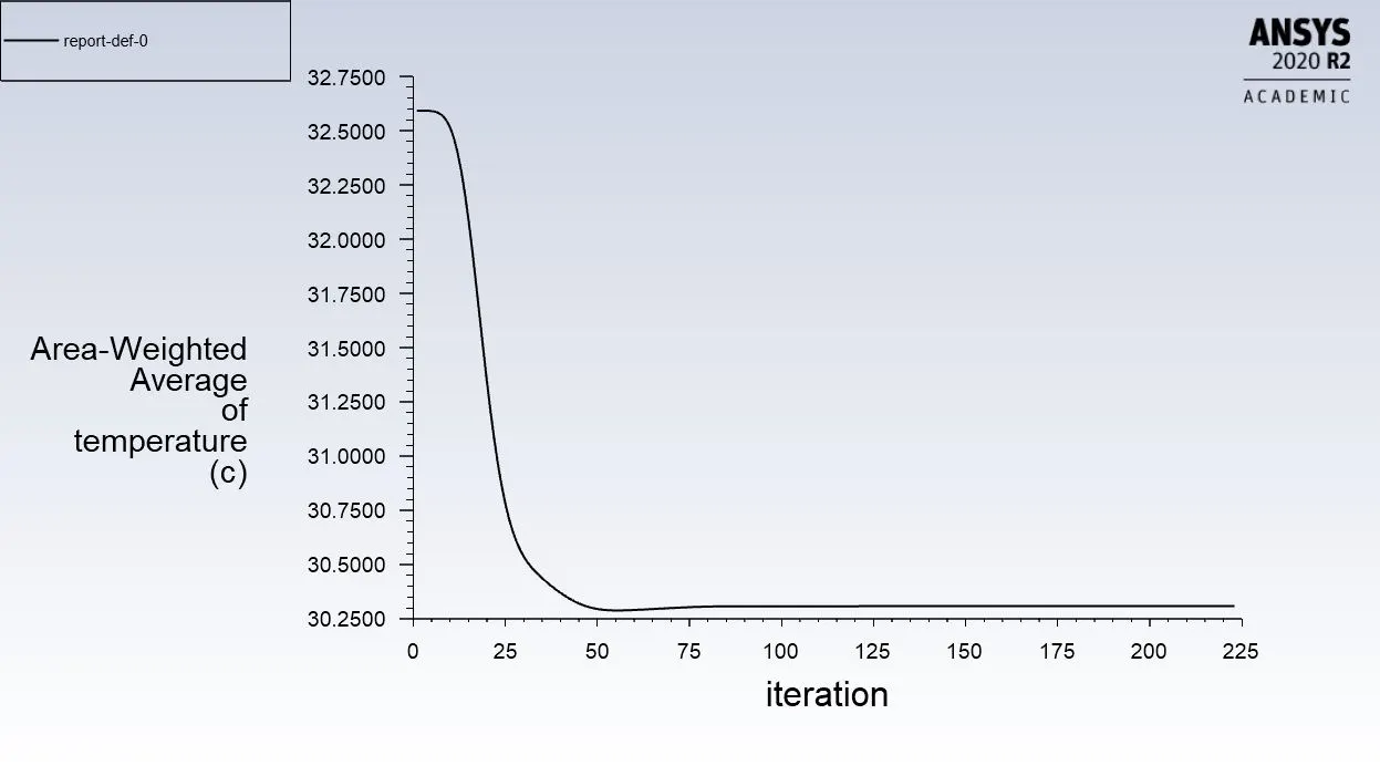
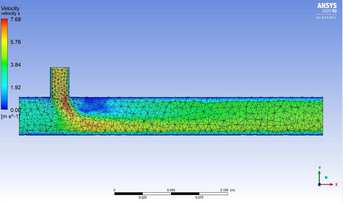
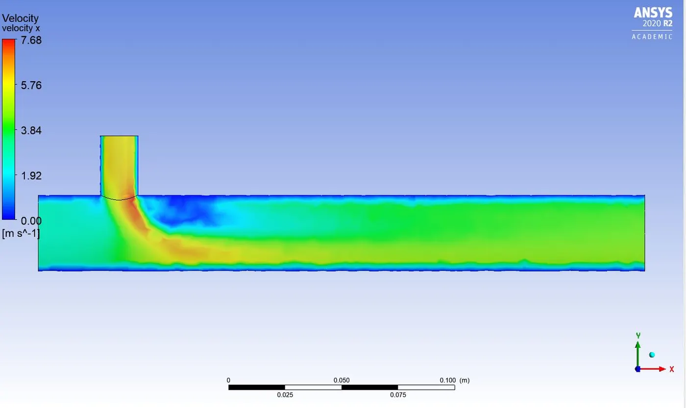
simulation: Post processing k epsilon long tee MR 2

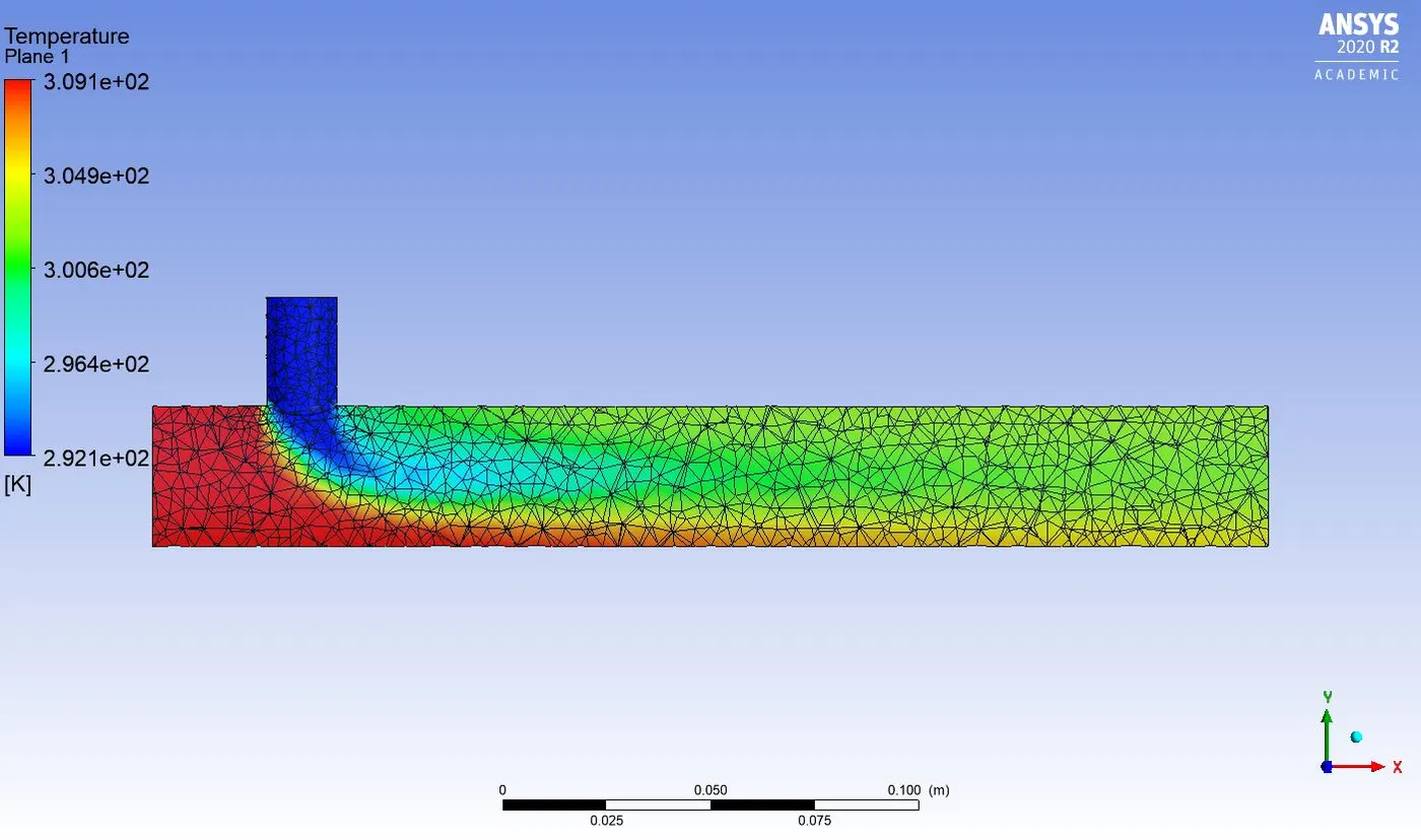
temperature contour MR2:

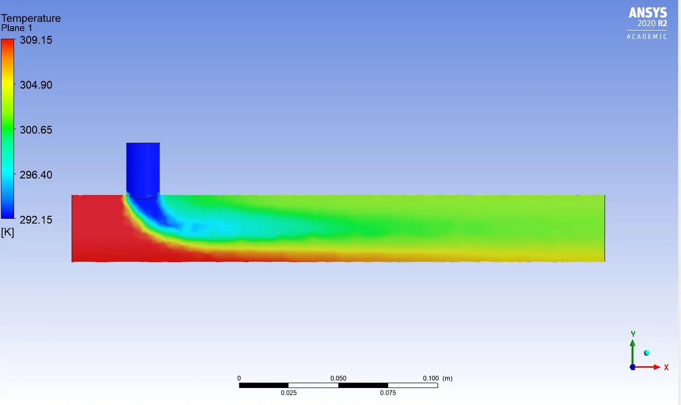
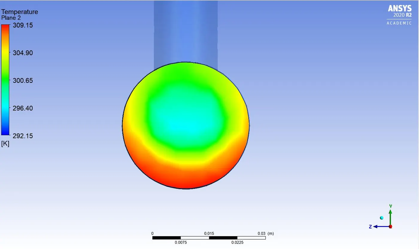
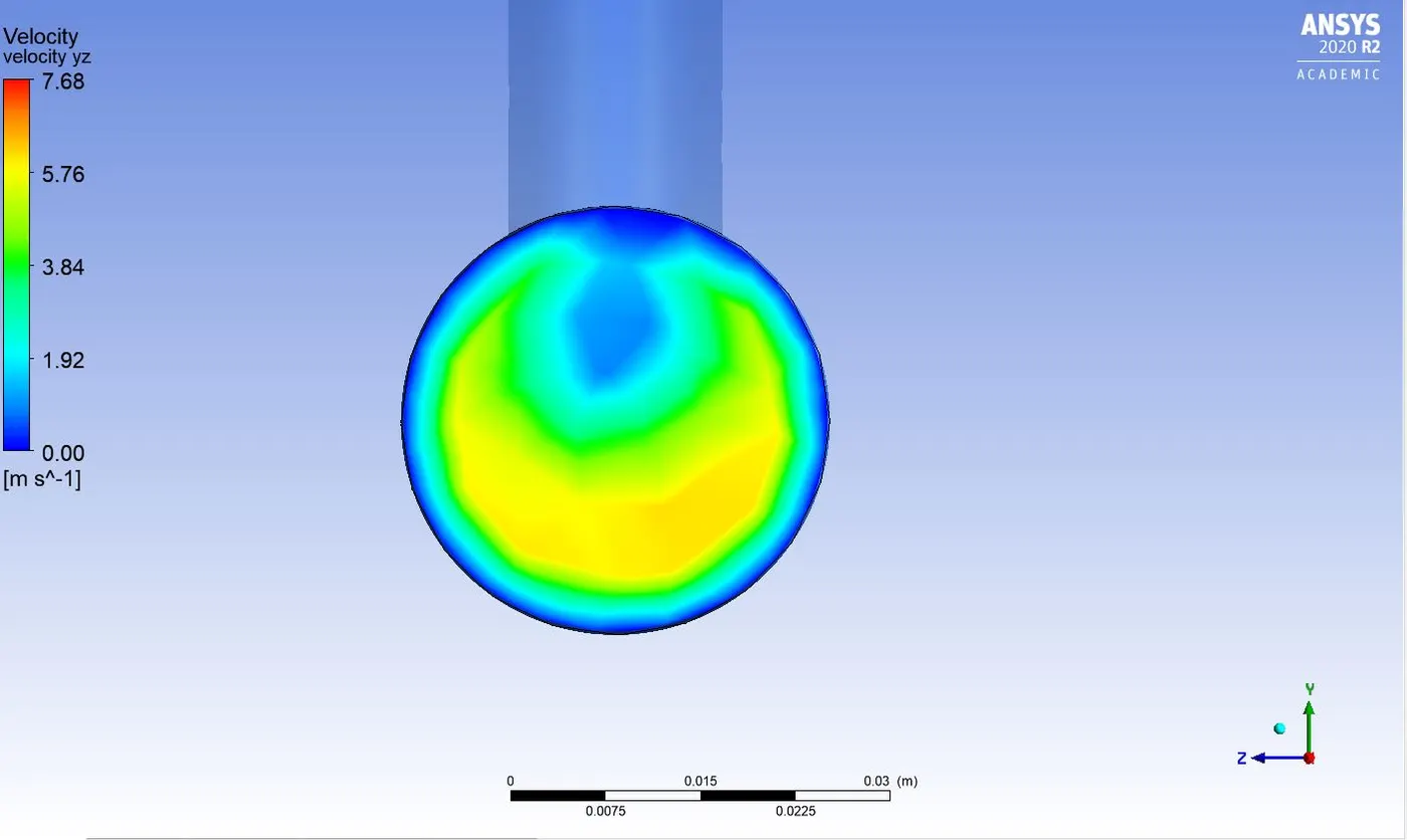
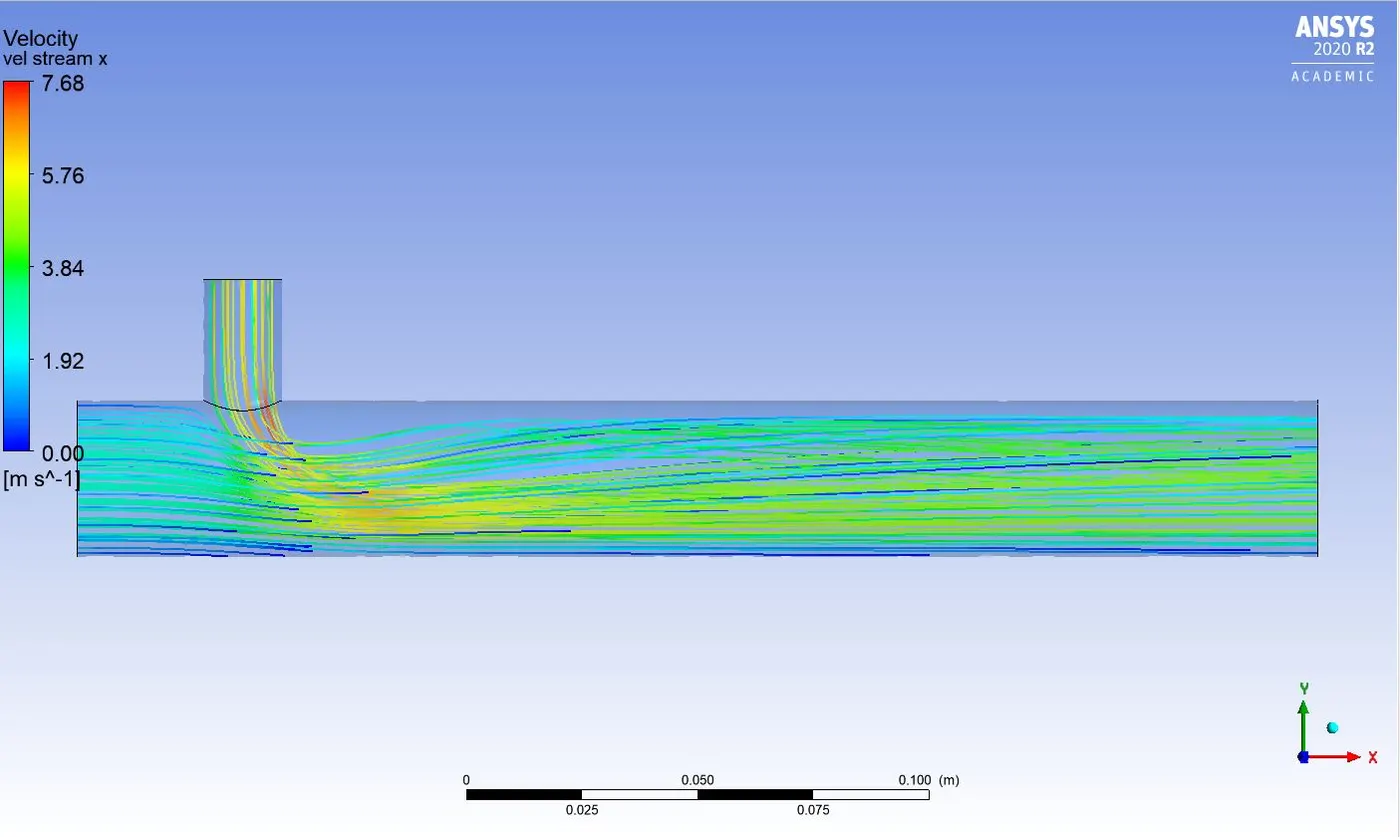
Velocity contours MR 2:

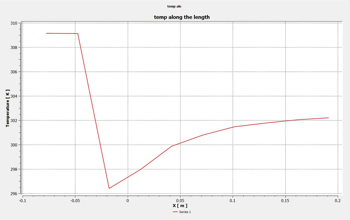
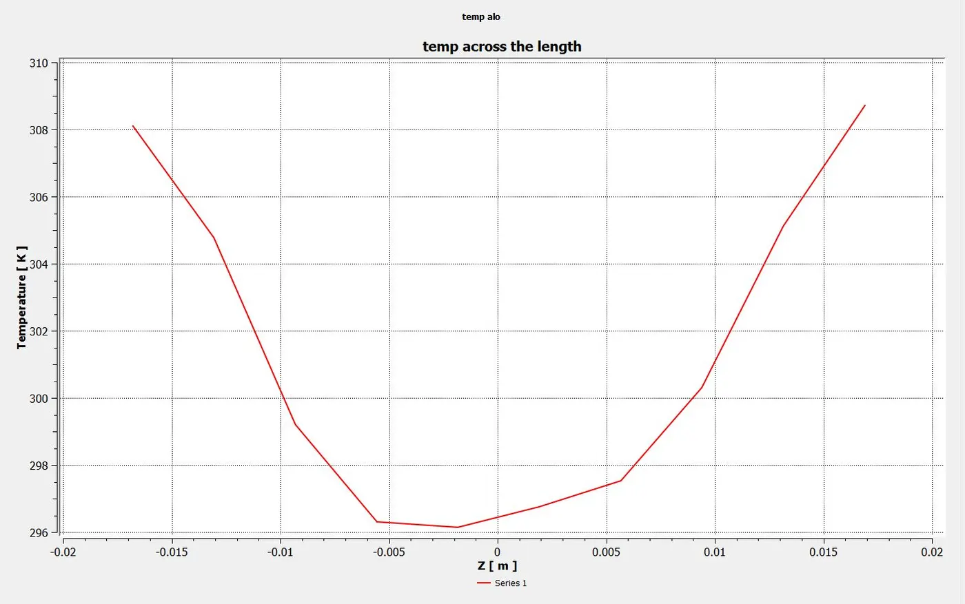
Temperature plot MR 2:

temp along the length: temp across the length

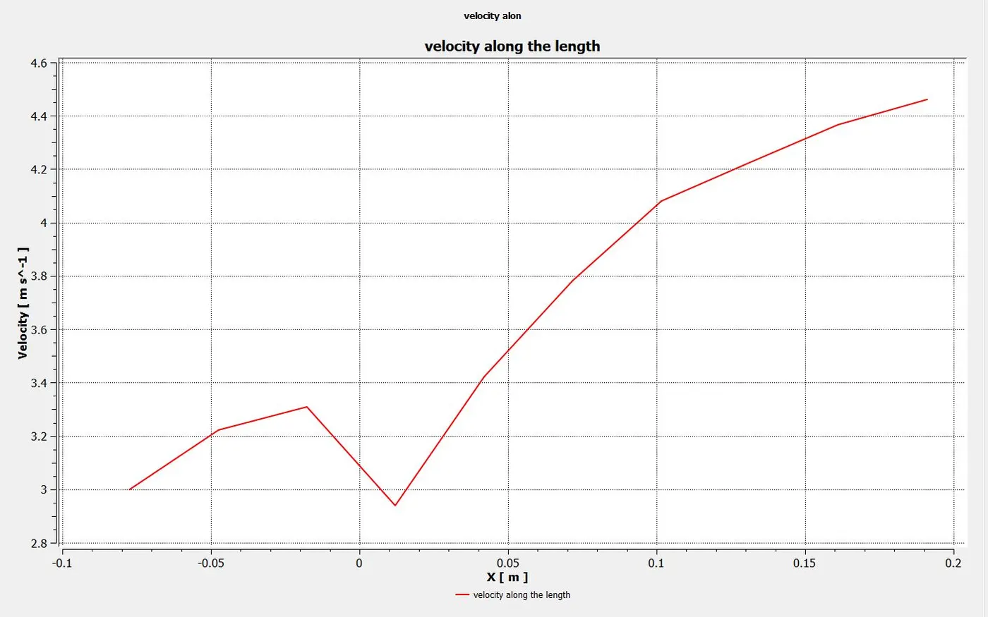
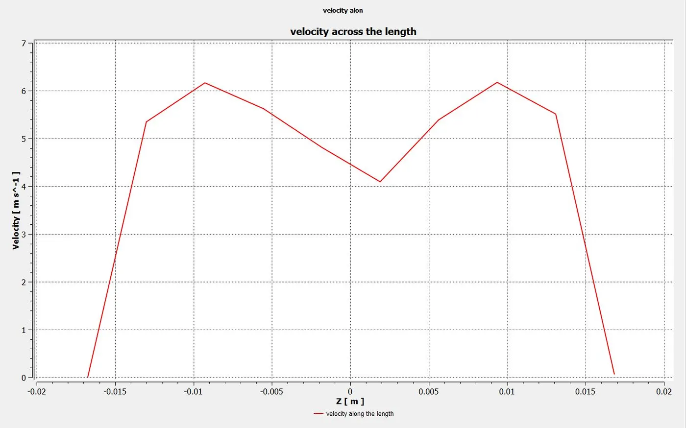
Velocity plot MR 2

velocity along the length: velocity across the length:

Momentum ratio 4:

Velocity inlet x=3m/s

velocity inlet y=12m/s

inlet temp x=36 degrees celsius

inlet temp y= 19 degrees celsius

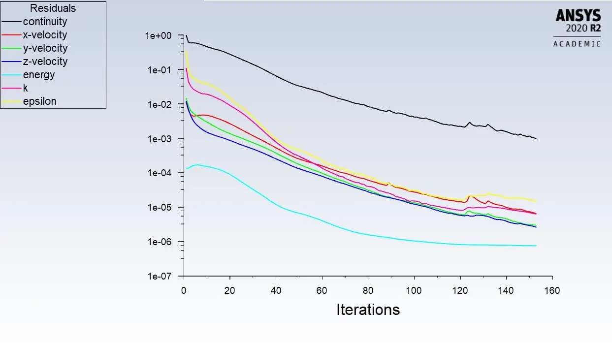
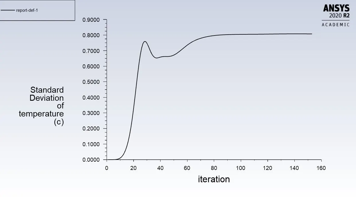
simulation: Post processing k epsilon long tee MR 4

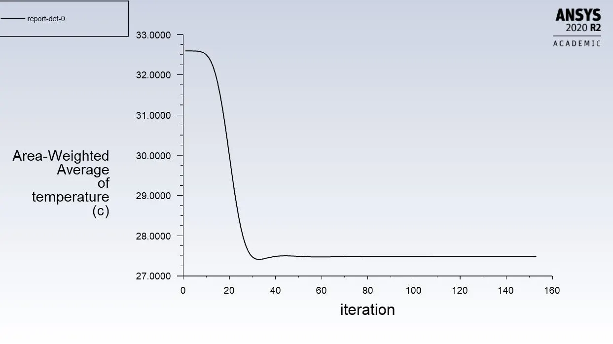
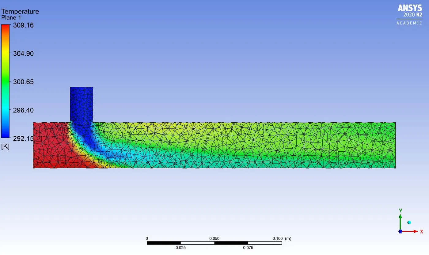
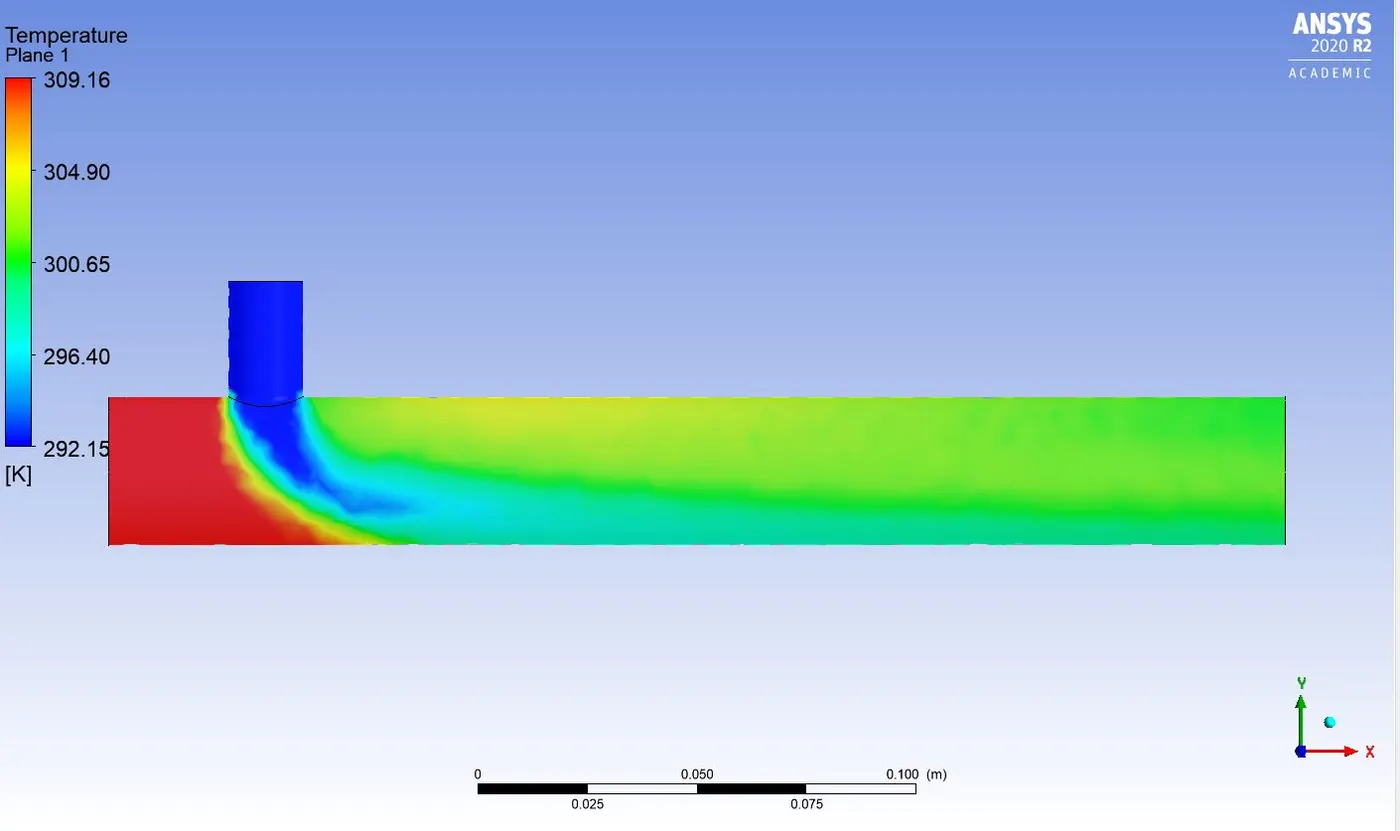
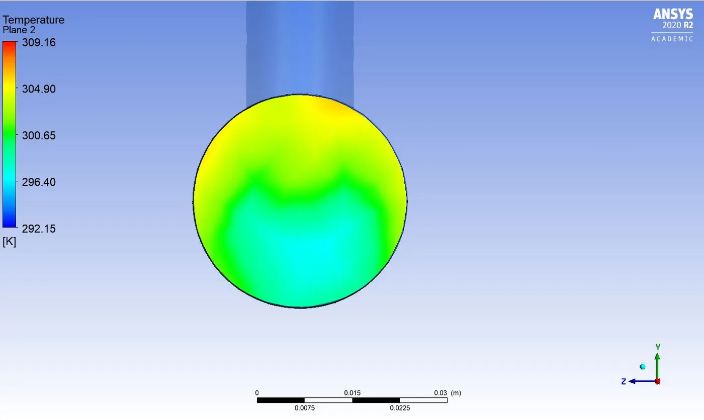
Temperature contour MR 4:

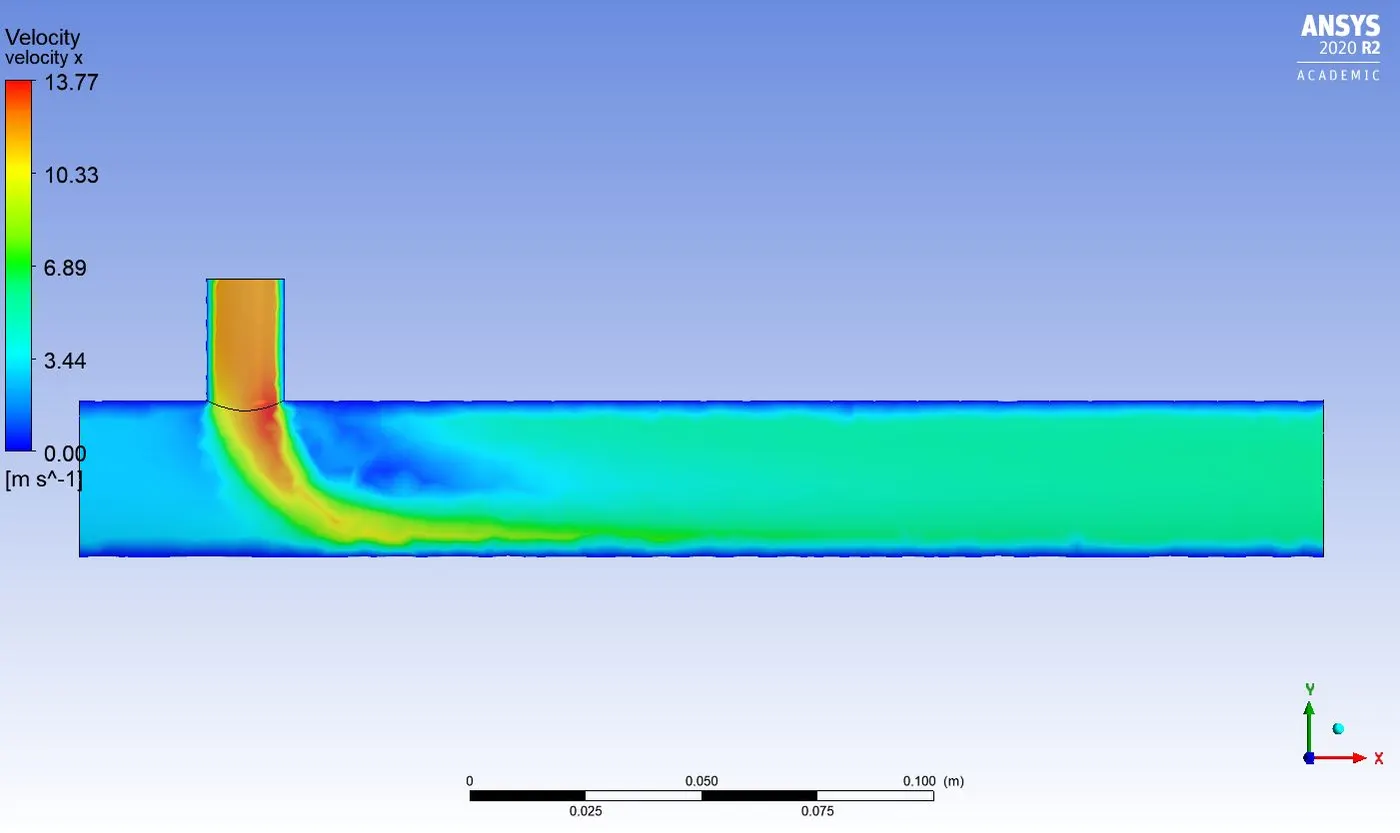
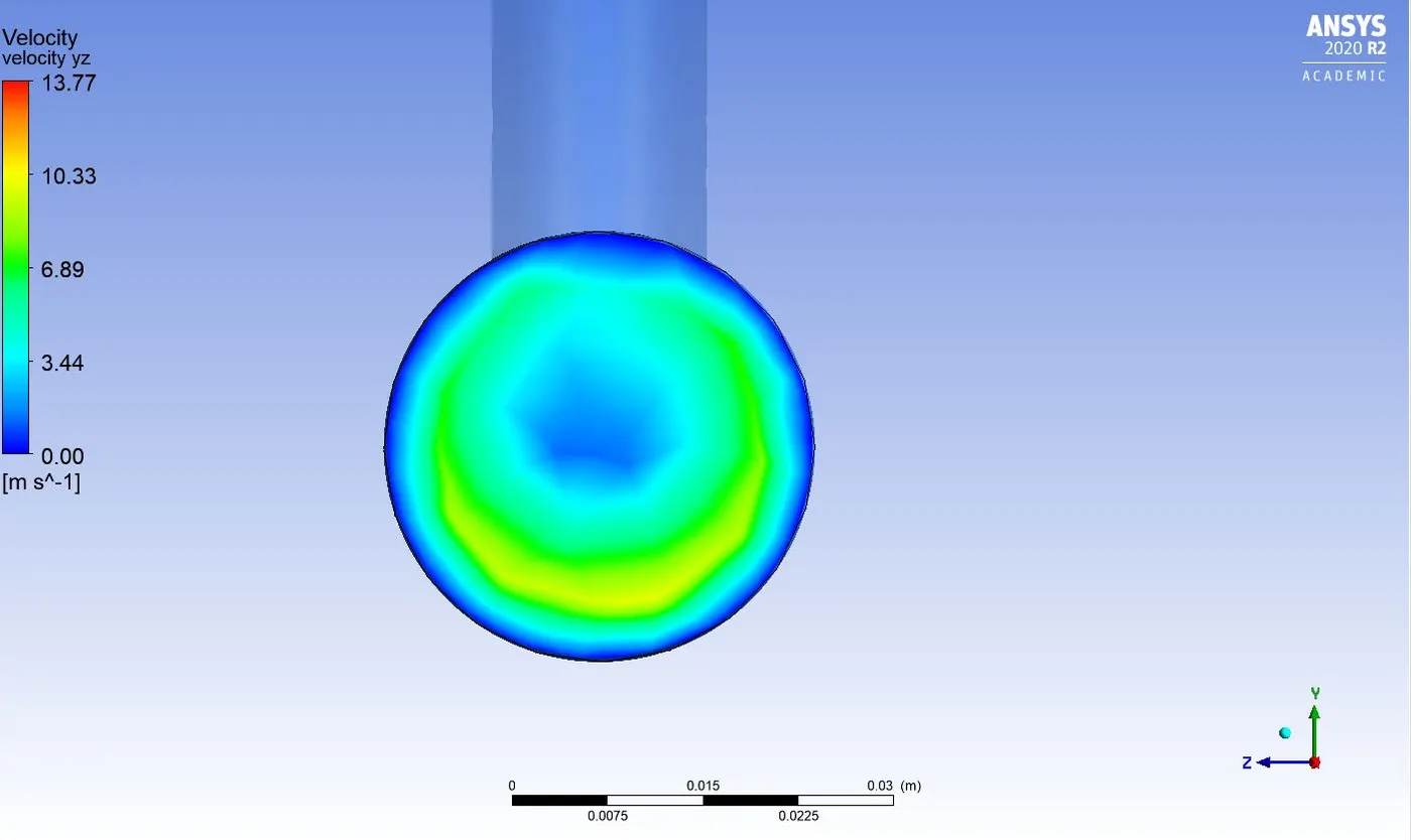
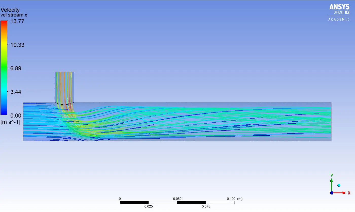
Velocity contour MR 4:

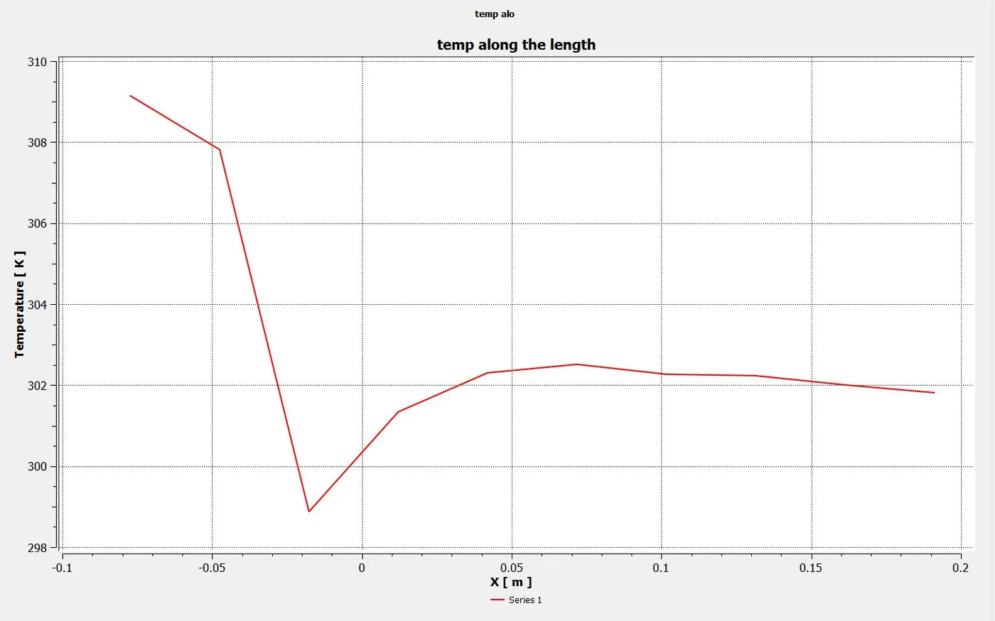
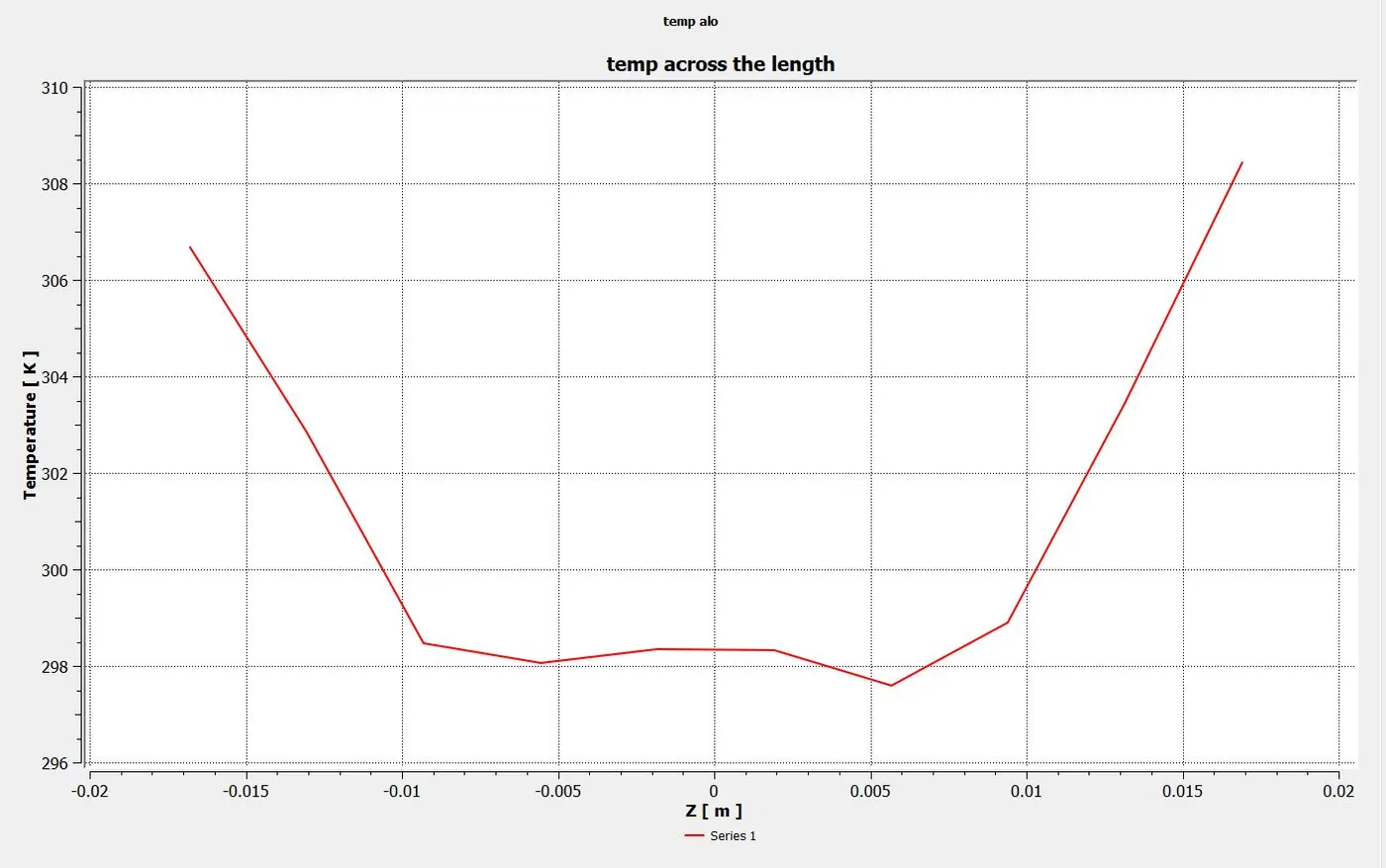
Temperature plot MR 4:

Temperature along the length: Temperature across the length:

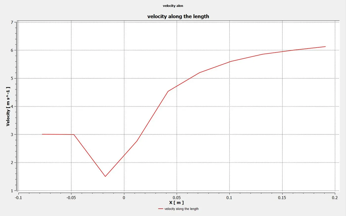
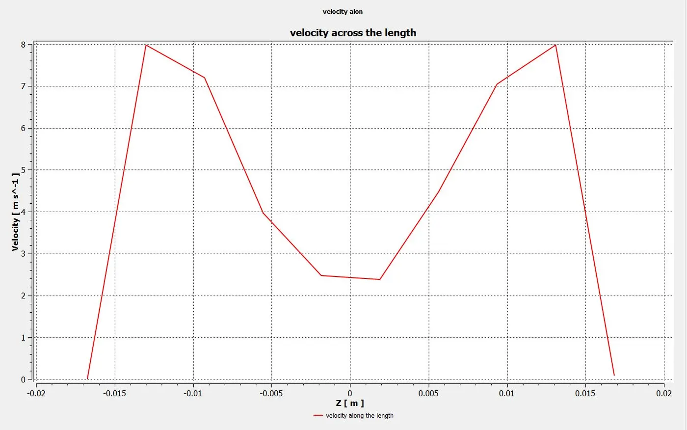
Velocity plot MR 4:

velocity along the length: velocity across the length:

comparison of results wrt to momentum ratio:

comparison of short tee and long tee k epsilon model

MESH INDEPENDENCY TEST:

For short tee MR 2

element size 5mm: element size 10 mm:

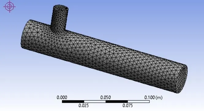
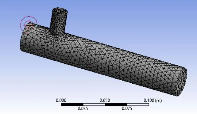
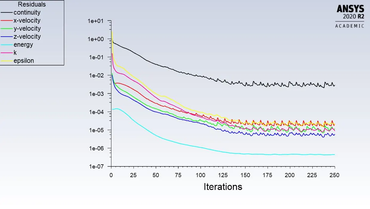
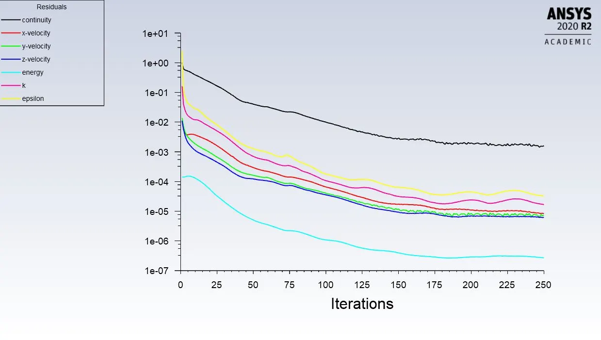
Residuals 5mm Residuals 10mm

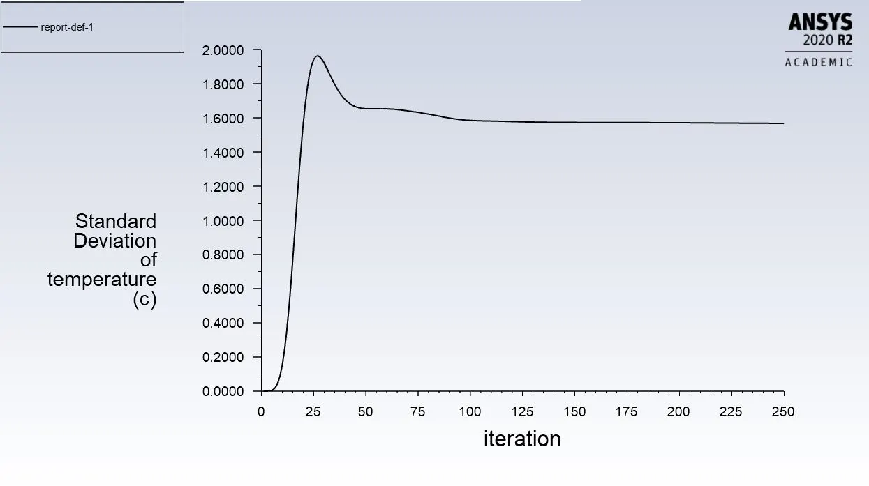
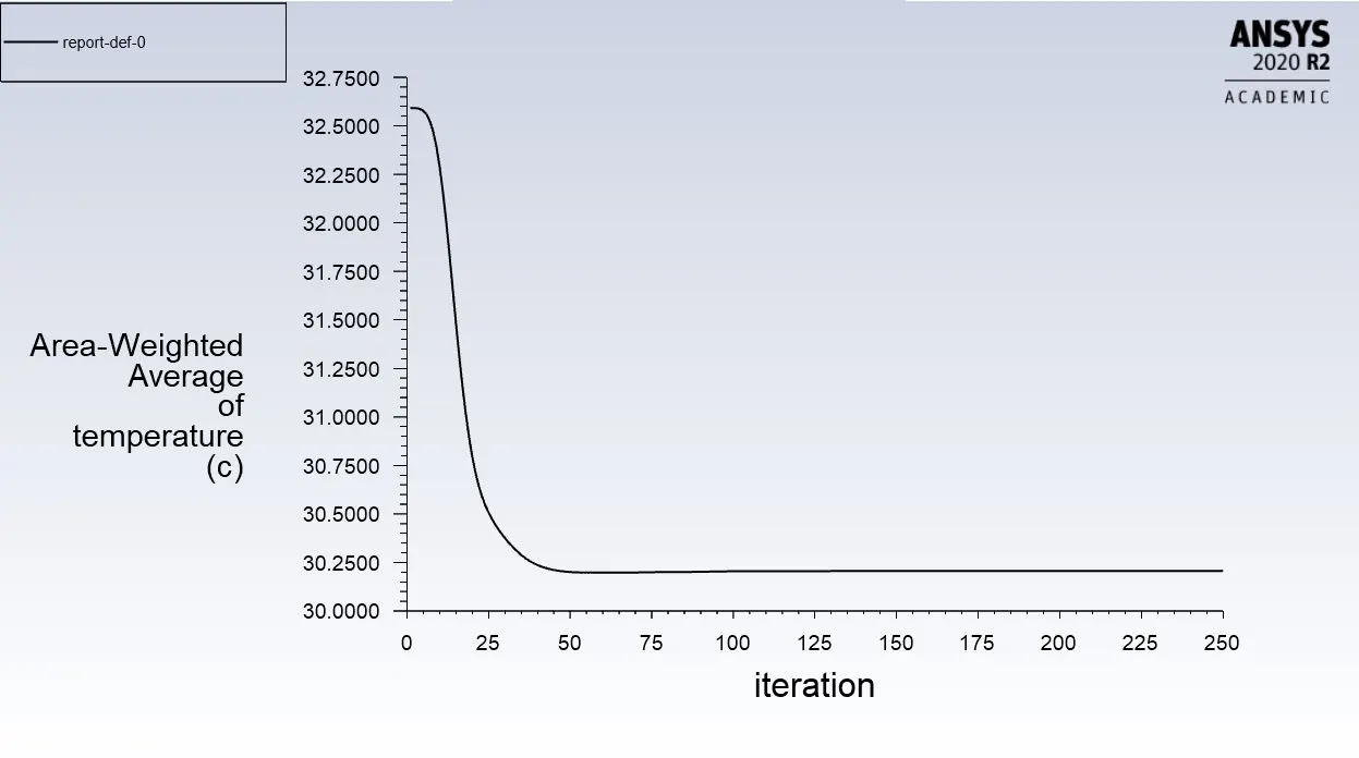
area weighted avg of temperature 5 mm area weighted avg of temperature 10 mm

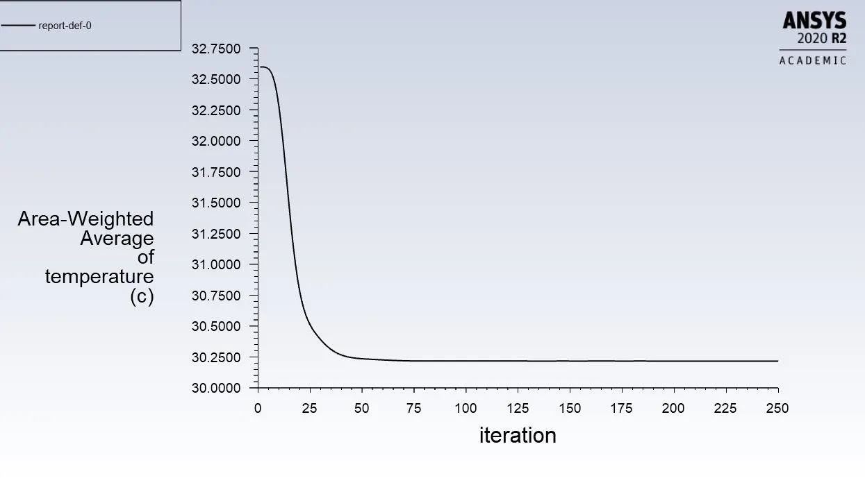
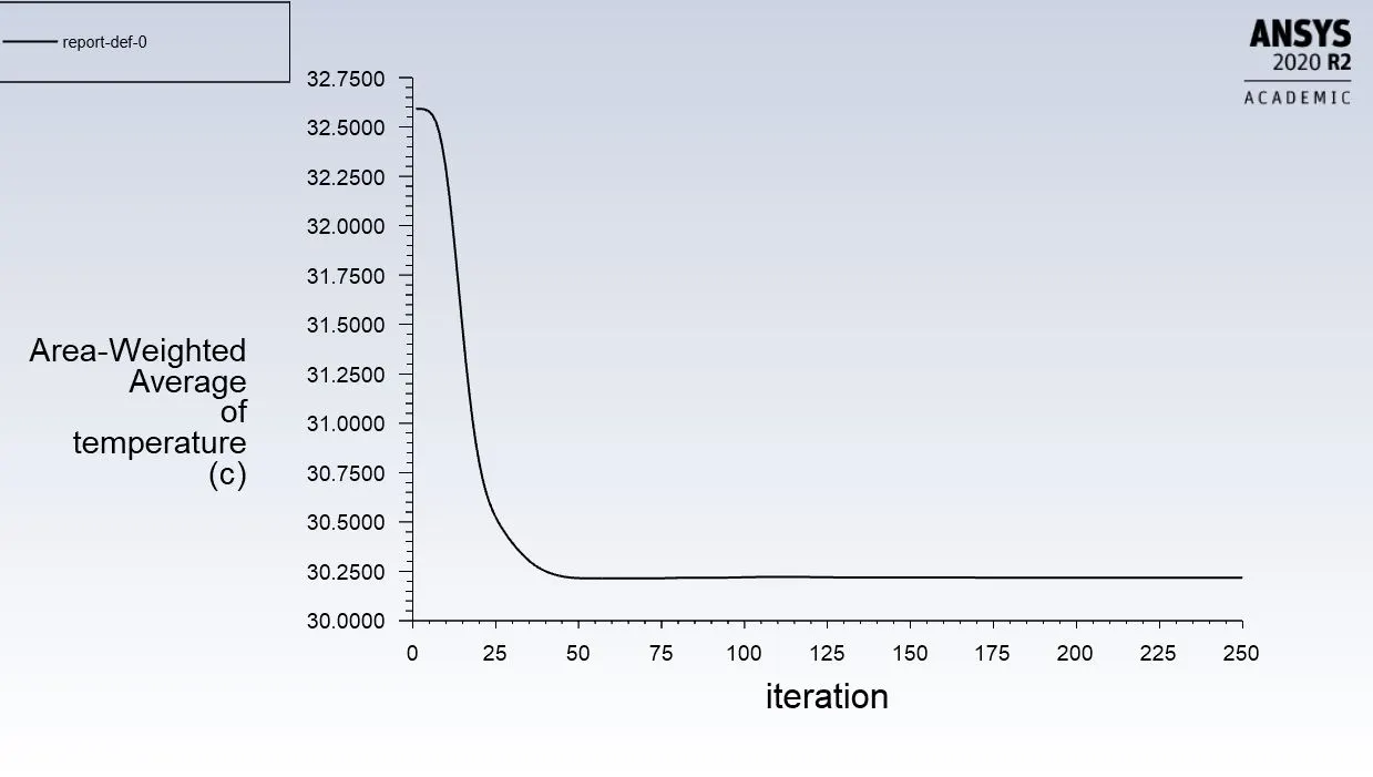
standard deviation of temperature 5mm standard deviation of temperature 10 mm

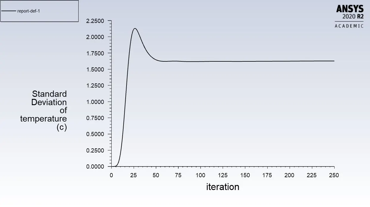
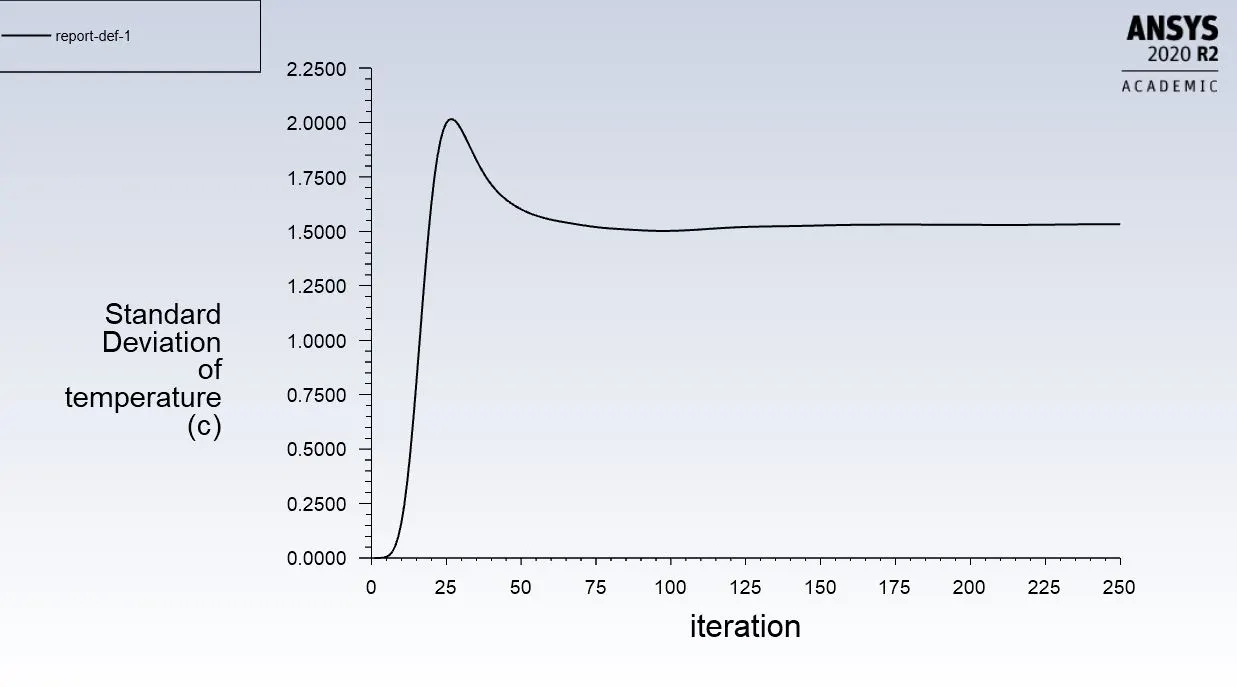
Mesh independency test table of comaprison between different size of short tee mixing

FINAL CONCLUSION:

• Smaller the mesh size better the accuracy but here in the case of short tee the difference is very small.
• For maximum mixing tee short tee with momentum ratio 4 is preferred by which we can converge to solution faster.
• in the k-epsilon model we can clearly see that the length of the pipe does not matter a lot but the momentum ratio i.e the speed of cold inlet matter a lot.
• for better mixing the velocity of inlet y (cold inlet) should be more.
• Momentum ratio tells about how behaviour changes by just changing the ratio so a lot of different ratios can be applied to obtain better mixing.
• standard deviation of long tee simulation is low by k epsilon model but the number of iteration are more so as part of computation power and accuracy we can decide to go with time aspects of simulation as in for complex geometry computational time matters a lot. And the standard deviation differece between the short tee and long tee for MR 4 is 0.04 which is not much of problem.

Summarizing the final conclusion:

For maximum mixing effeciency higher momentum ratio MR 4 is preferred which has higher cold inlet velocity and is good for both short and long tee models especially with short tee to save computational power.