Exhaust Port Challenge
Aim: To simualate the conjugate heat transfer on a Exhaust port.
Objectives:
- To understand why and where a Conjugate heat transfer(CHT) analysis is used.
- To maintain the y+ value according to the turbulence model and justify the results.
- To calculate the wall/surface heat transfer coefficient on the internal solid surface & show the velocity & temperature contours in appropriate areas.
- To verify the heat transfer coefficient predicted values for simulation.
- To dertermine the factors on which the heat transfer coefficient prediction depend on.
Theory:
Conjugate Heat transfer:
The term conjugate heat transfer (CHT) is used to describe processes which involve variation of temperature within solids and fluids because of thermal interaction between solids and fluids.The rate of heat transfer is directly proportional to the temperature difference. In solids the conduction dominates and in fluids convection dominates. Efficiently combining both fluids and solids is a key to design any heat involving machine.
Heat transfer in solids and heat transfer in fluids are combined in majority of applications. This is because fluid flow around solids and the fact that solids are immersed in fluid. For example a hot cup of water is surrounded by ambient air. The basic crux of applying CHT analysis is getting understanding for how can we incorporate a solid and fluid interactions with required amount of heat transfer between them.
CHT analysis is used in many application for mainly cooling purposes like radiators,water jackets in ic engines,battery pack cooling. Basically where ever we can find solid and fluid volume in conjuction.
Modelling approch and solving:
- First we need to extract the volume and make two volumes , fluid volume and solid volume
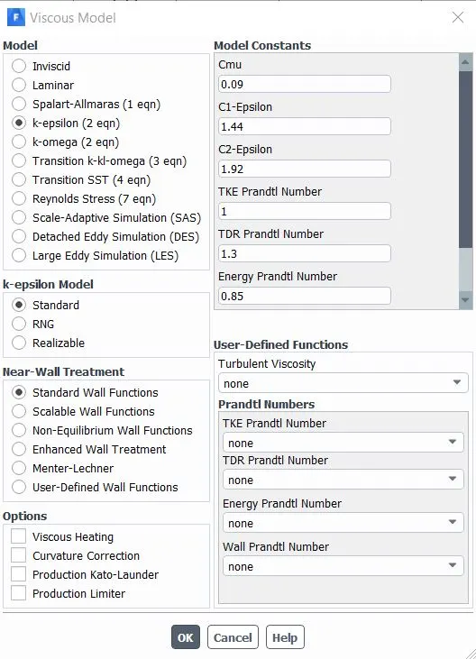
- Next we build up three cases which constitute one k-epsilon simulation and other two k-omega sst simualation.
- k-epsilon constitute a coarse mesh(baseline mesh k- epsilon)
- k-omega constitue a coarse mesh(baseline mesh k-omega)
- k-omega refined mesh with inflation layers.
- Choice of turbuolence model is k-omega sst in order to capture the near boundary simulation.
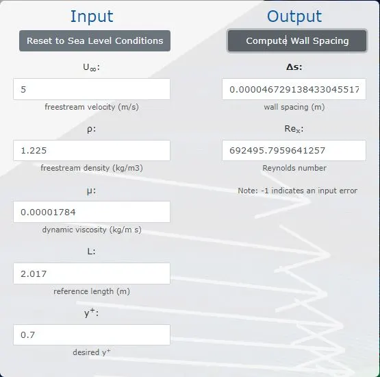
- calculation of y+ value based on k-omega sst model.
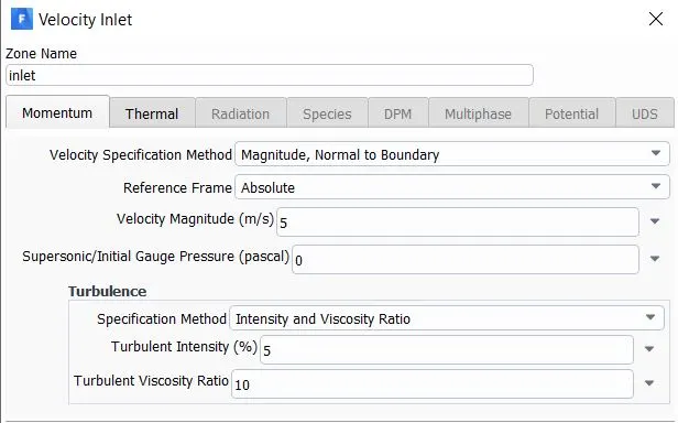
- solving in fluent by using pressure based steady state solver using boundary condition.

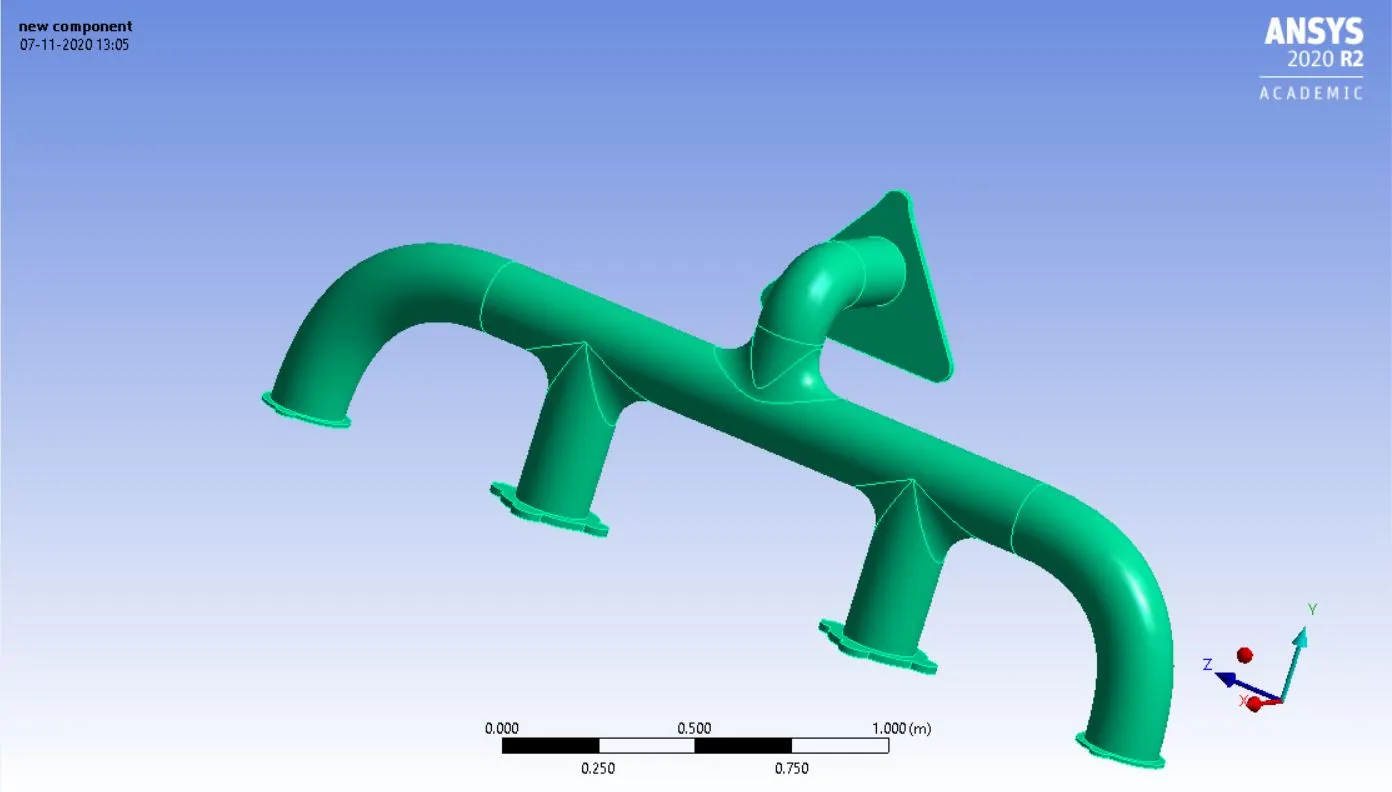
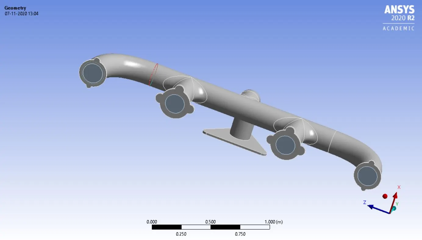
Geometry:
The geometry is a volume extracted preapared for simulating CHT.
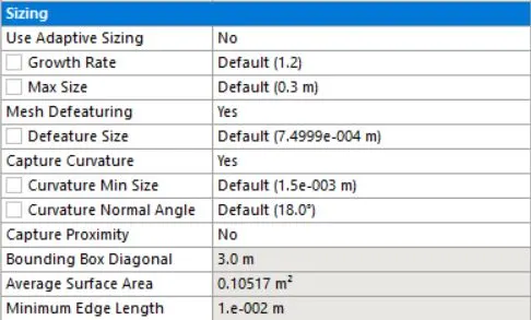
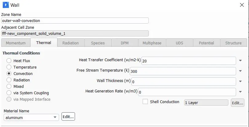
------------------------------------------------------------------------------------------Case 1: Baseline mesh with k-epsilon model---------------------------------------------------

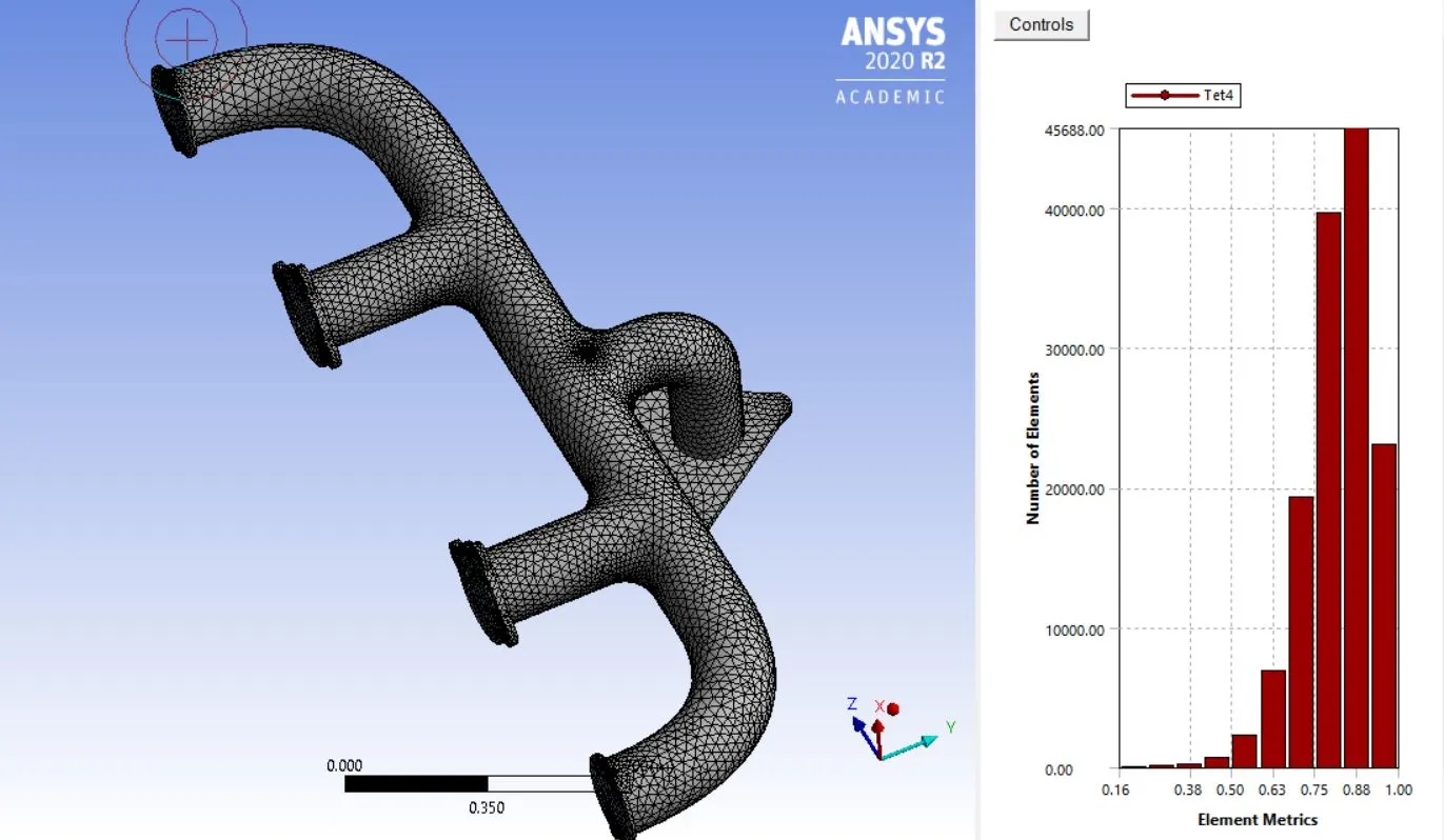
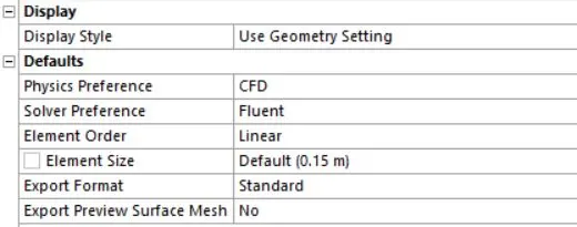
Meshing:

Fleunt setup:
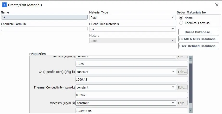
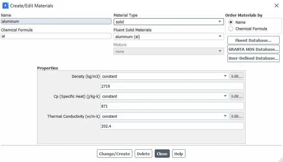
Material properties:
Results of pre and post processing:
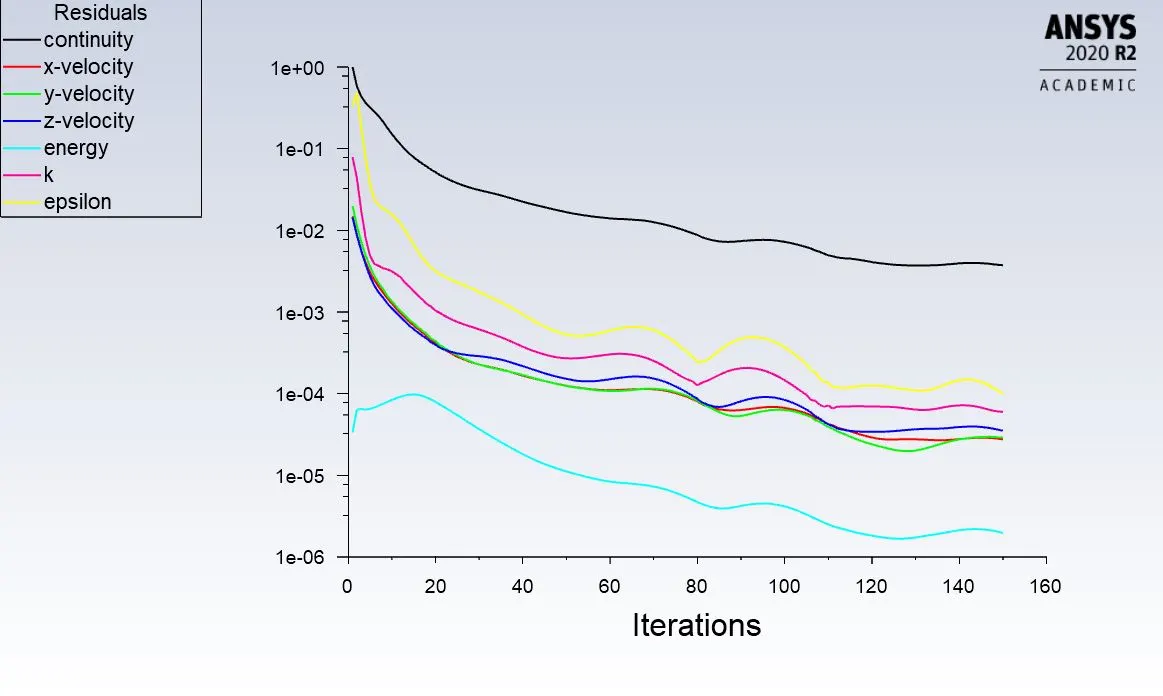
Residuals:
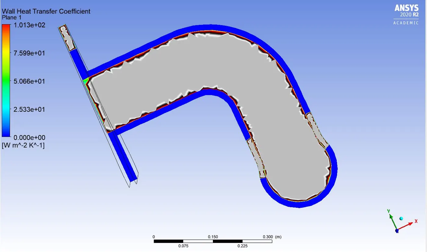
Wall heat transfer coefficient:
velocity contour:
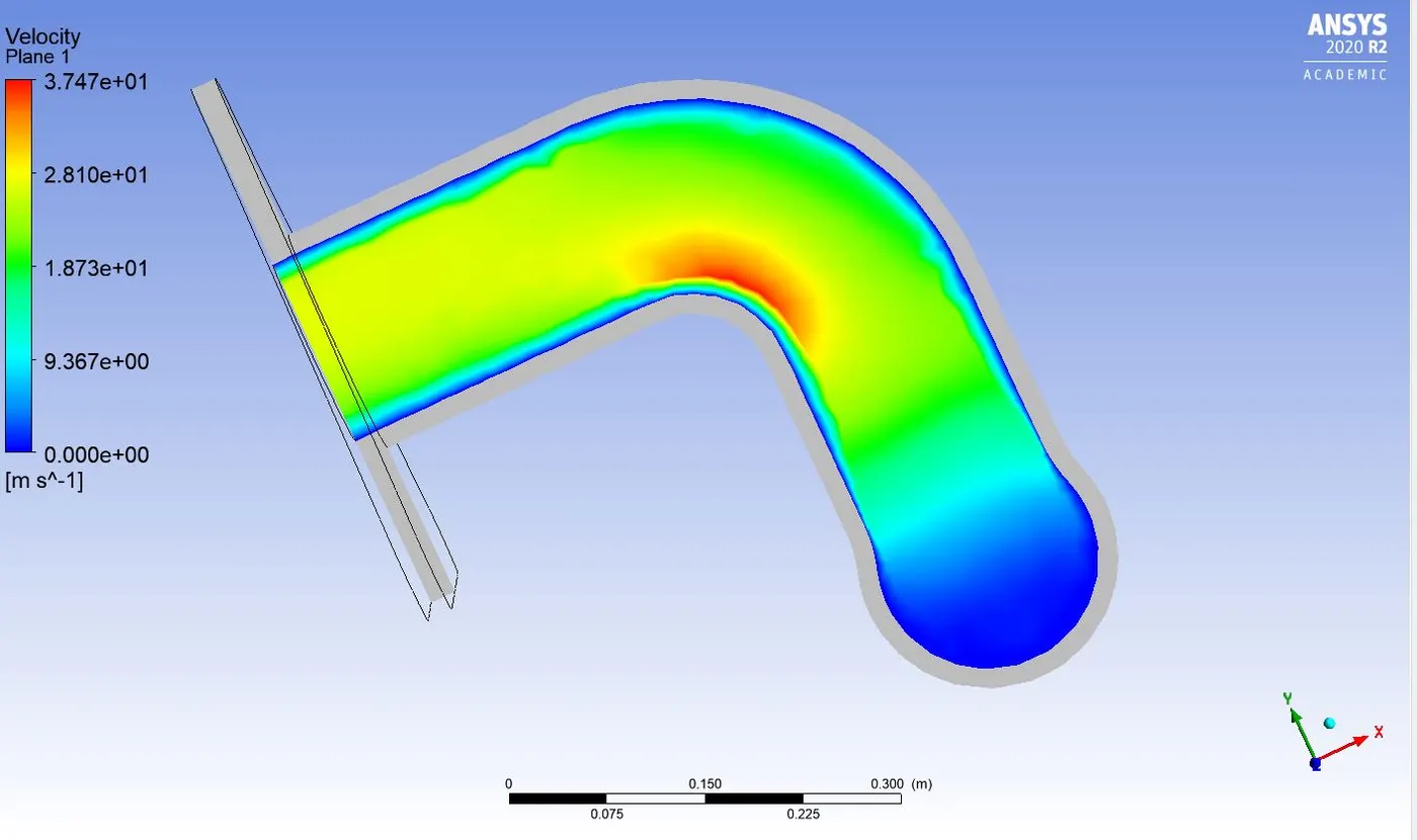
Temperature contour:
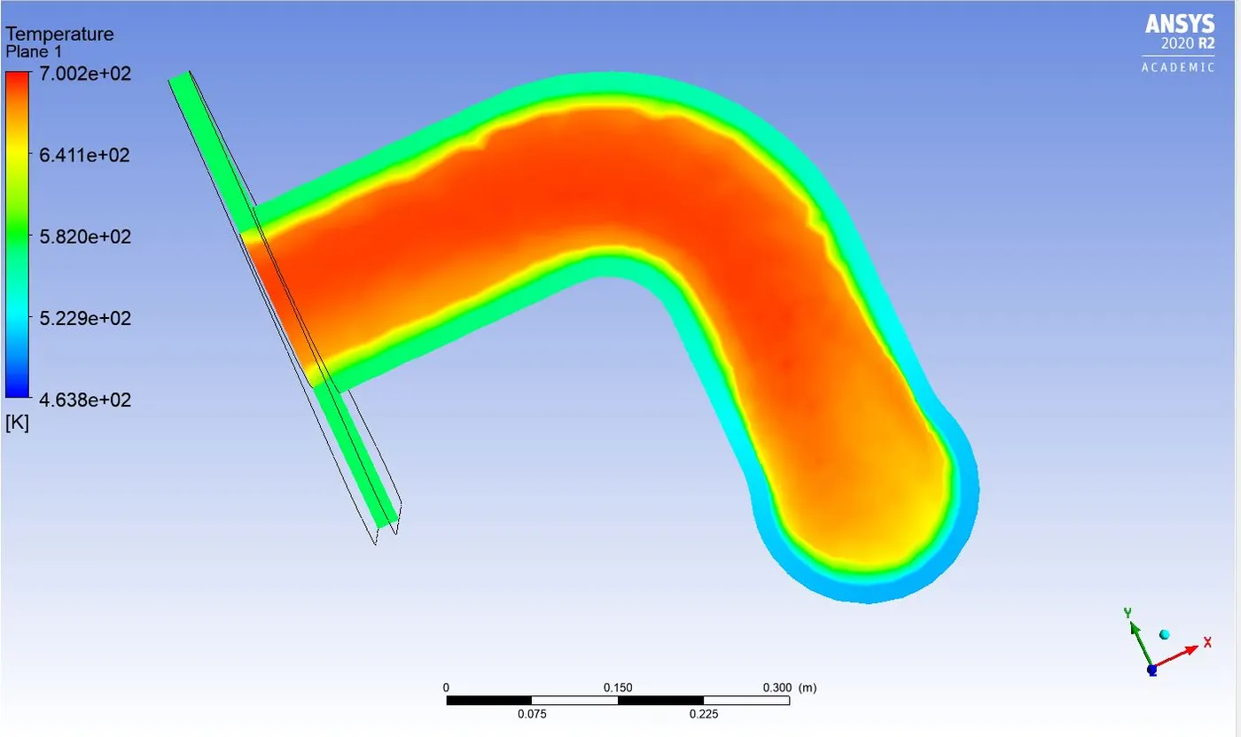
streamlines:
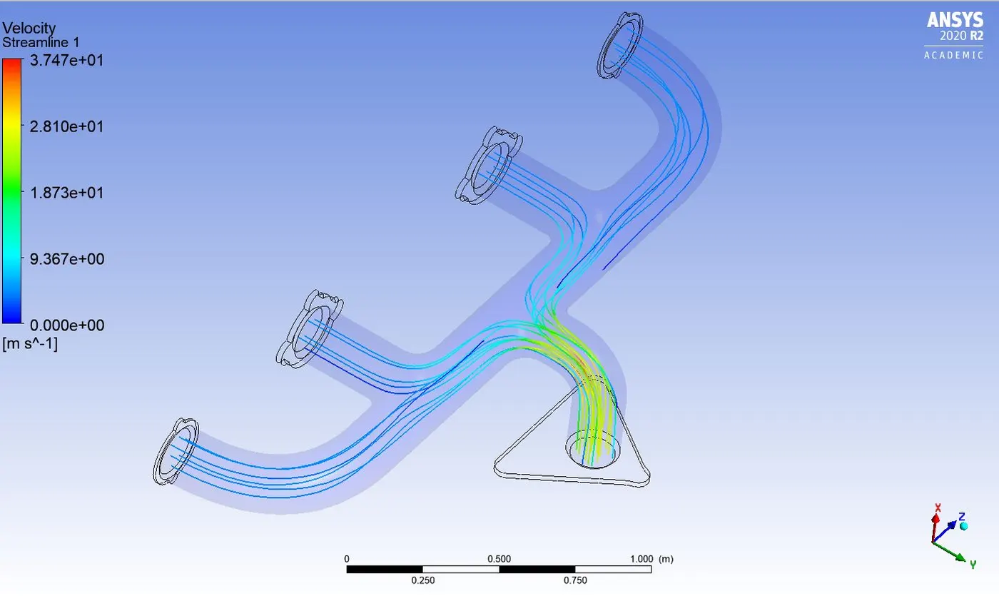
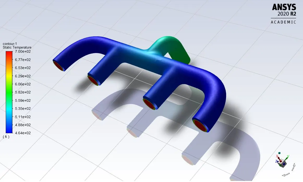
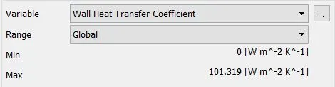
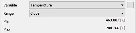
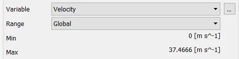
Results table

------------------------------------------------------------------------------------Case 2 : Baseline mesh with K-Omega model--------------------------------------------------------------------------------------

Note:
Mesh : The model and mesh sizing is same as that of case 1
Fluent setup:
k-omega sst model
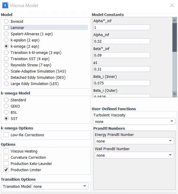
Note : other properties like material and boundary conditions are same as case 1
Results of pre and post processing:
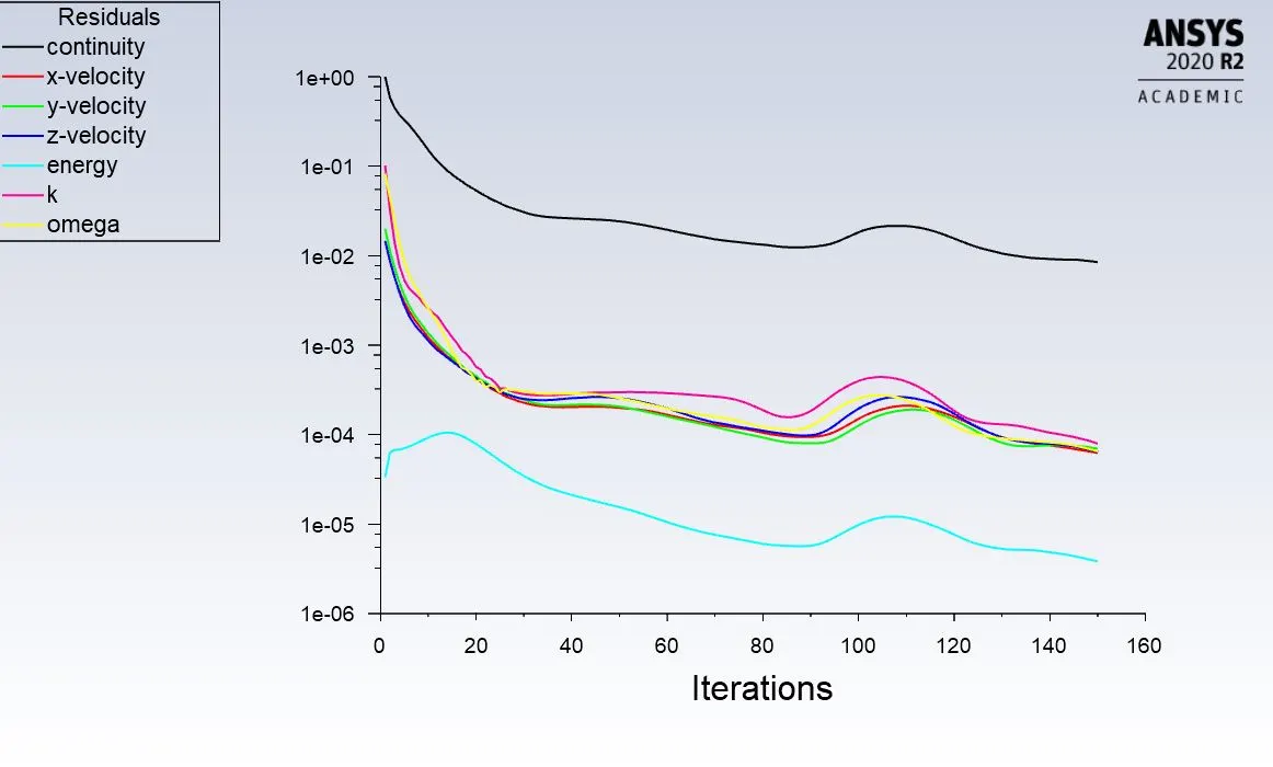
Residuals:
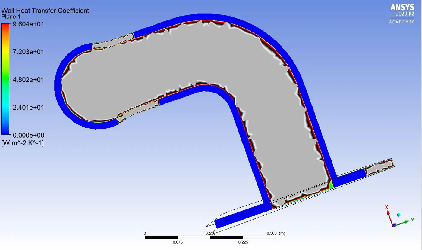
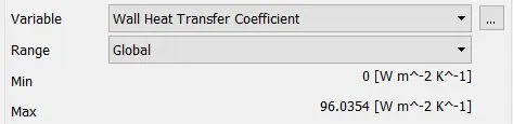
Wall heat transfer coefficient:
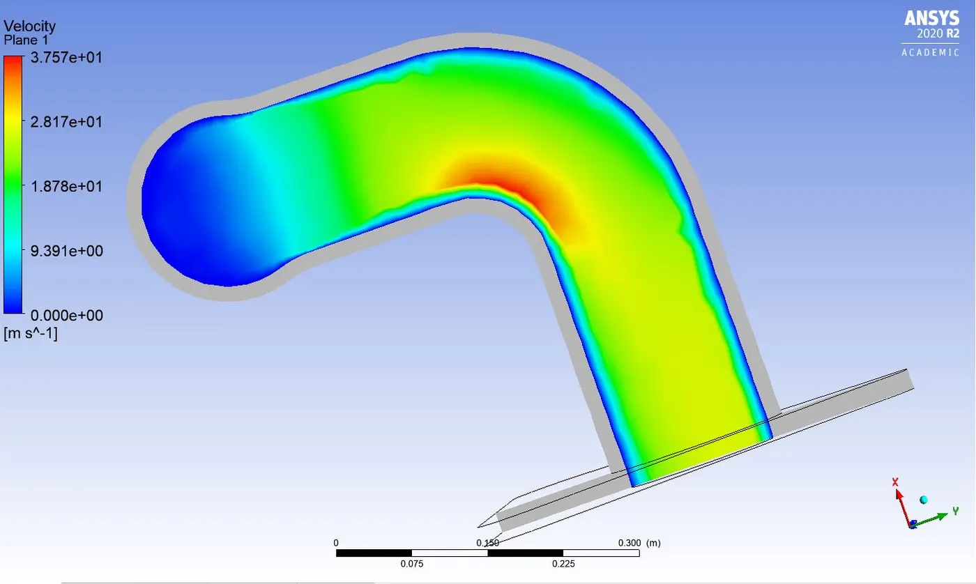
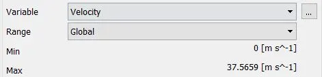
velocity contour:
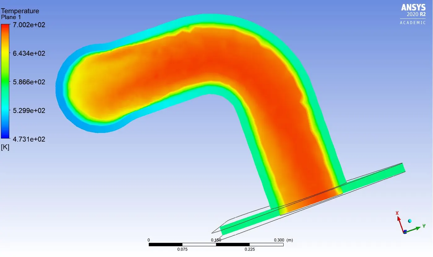
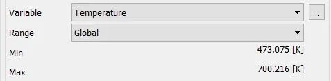
Temperture contour:
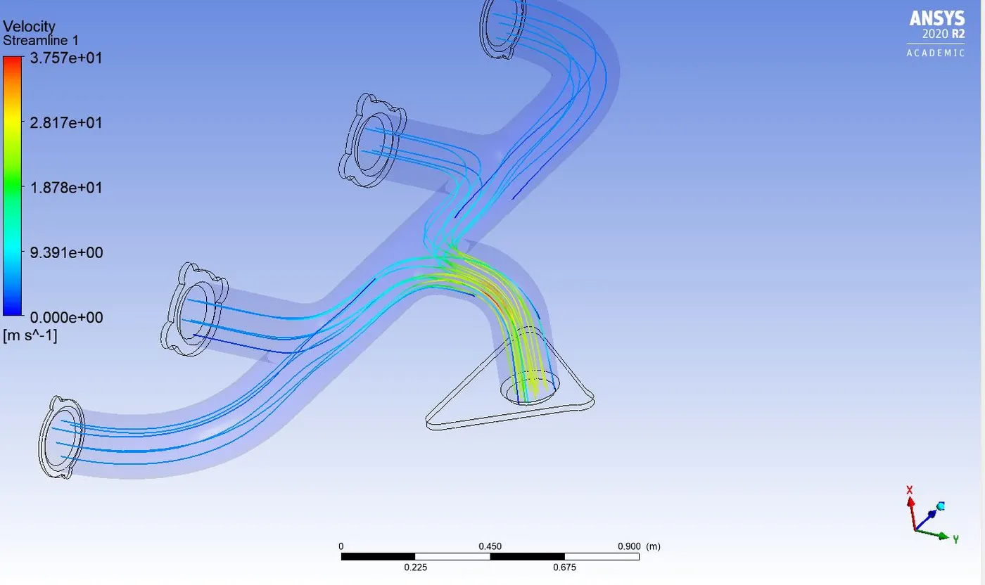
Velocity streamlines:
Result table case 2:

--------------------------------------------------------------------------------Case 3: Refined mesh with inflation K-Omega sst model-----------------------------------------------------------------------------------

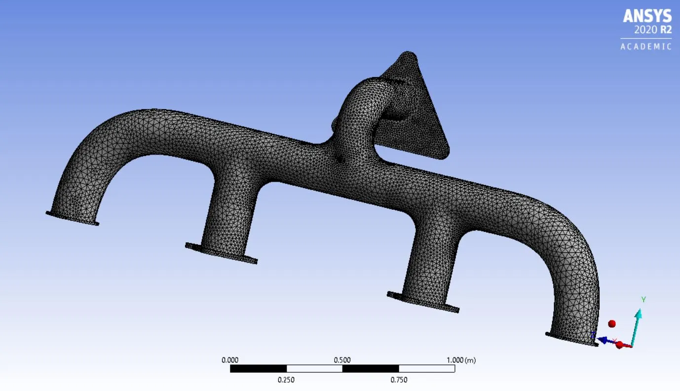
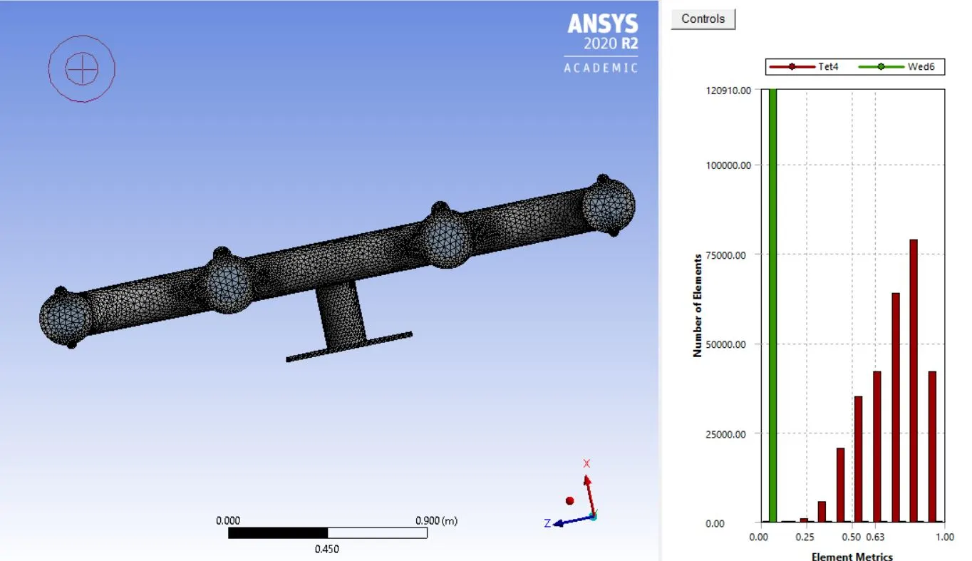
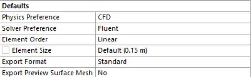
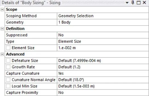
Mesh :
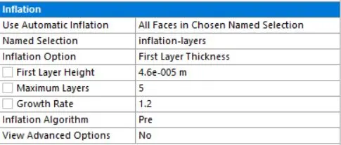
Inflation layer:

Fleunt setup:
k omega sst
pressure based solver
inlet velocity 5m/s
heat transfer coefficient h=20 w/m^2.K
outlet is pressure outlet is gauge pressure.
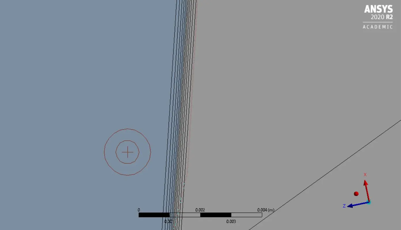
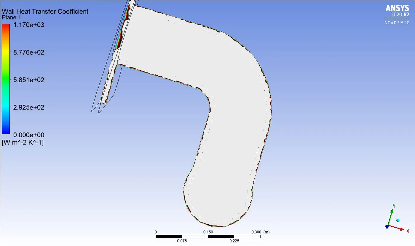
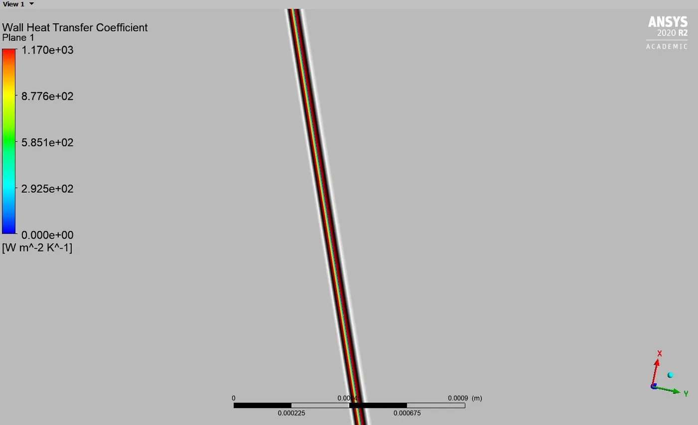
Y+ value is 0.7 with first layer thickness is 0.000046m
Results of pre and post processing:
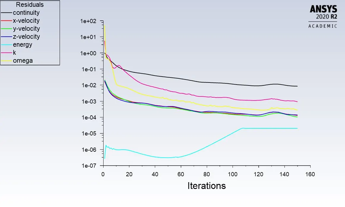
Residuals:
wall heat transfer coefficient:
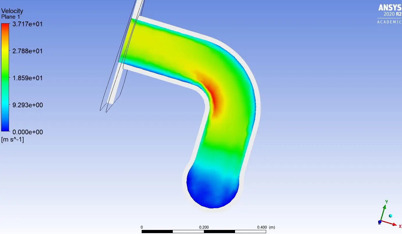
velocity contour:
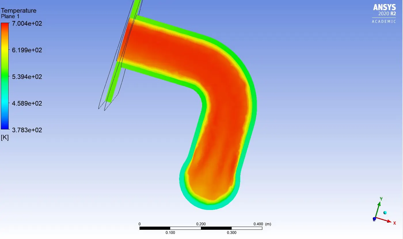
temperature contour:
Results:
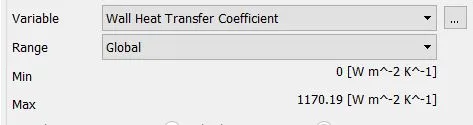
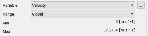
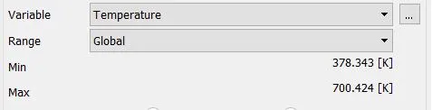
Results table

-----------------------------------------------------------------------------------------------------------------------------------------------------------------------------------------------------------------------------------------
Overall Results:

Verify the HTC predictions from the simulation are right and on what factors the accuracy of prediction depend upon:
Heat transfer coefficeint in convection can be quantitatively calculated on paper as it depends upon temperature difference and nusselts number.
Nusselts number `Nu= (hl)/k` l=length, h= heat transfer coefficient and k is the thermal conductivity of material.
To calculate the heat transfer coefficeint we calculate the nusselts number. This can be done by dittuis bolter equation.
`Nu= A.(Re)^b.(pr)^c`
A,b and c values varies and depends on dimension of model
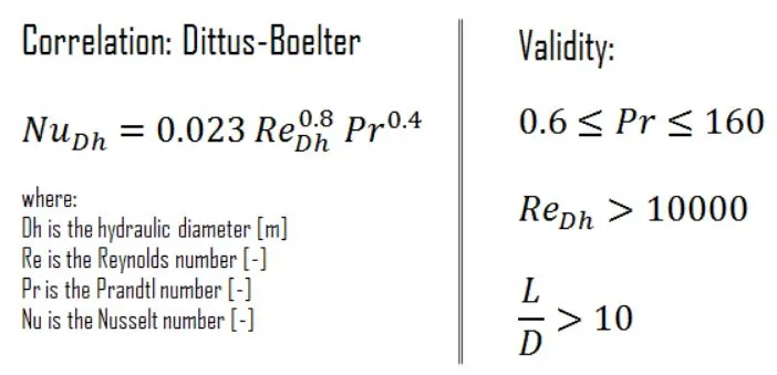
since the reynolds number is greater than 10000 and the dittus boelter equation can be validated to summarize the accuracy of predictions
Other way of verifying is by grid dependency test . By making a table of different grid sizes, y+ values and simulating the values for heat transfer coefficient we can come upto some understanding to predict the value.
Factors on what the accuracy of predictions are based upon:
- choosing the turbulence model like k-omega sst which gives better results at wall.
- choosing y+ values.
- Mesh quality is another factor which can increase the accuracy.
- more refined mesh can give better prediction of HTC which will certainly increase the element size
- inflation layers plays an important role in giving an accurate value.
Inferences and conclusion:
- wall heat tranfer coefficeint can be a tricky value and experimental analysis can really give better results.
- we can infer that that the boundary anlaysis and the y+ calculation results better way of capturing the near wall heat transfer.
- from the final table can see that the rate of heat tranfer is way better for k omega sst model with inflation layers
- Greater the temperature difference the rate of heat tranfer is more.
- There is a huge upgrade from baseline mesh of k -omega to refined mesh with inflation layer which gives a far more better results.
- The temperature and velocity contour of refined mesh setup give accurate contour than the baseline mesh