Rayleigh Taylor Instability Challenge
Aim: To perform Rayleighs taylor instability by using two different material primarily water and air.
Objectives:
- Explanation of practical CFD models that are based on mathematical analysis of Rayleighs Taylor waves.
- Perform RT instability anlaysis using Volume of fraction model on two different mesh sizes and compare the results with animations.
- Perform the similar analysis using water and user defined material (rho=400 kg/m^3;mu=0.001 kg/ms)
- Calculating the Atwood number in above cases and explain the how Atwood number affect the instability.
Theory:
Rayleigh-Taylor instability:
RT instability is an instabililty of an interface between two fluids of different densities which occurs when the lighter fluid is pushing the heavier fluid . Example include the behaviour of water suspended above the oil in the gravity of earth, mushroom clouds like those from volcanic eruptions and atmospheric nuclear explosion.
Water suspended on top of oil is an everyday example of RT instability , and it may be modeled by two completely plane parallel layers of immiscible fluid , the more dense on the top of less dense and both subject to earth's gravity. The equilibrium in this case is unstable to any disturbances of the interface. If a parallel of fluid is displaced downward with an equal volume of lighter fluid displaced upwards, the potential energy of the configuration is lower than the initial state and the disturbance grows and lead to further release of the potential energy . The movement of denser material moving up and down was studied by Rayleigh.
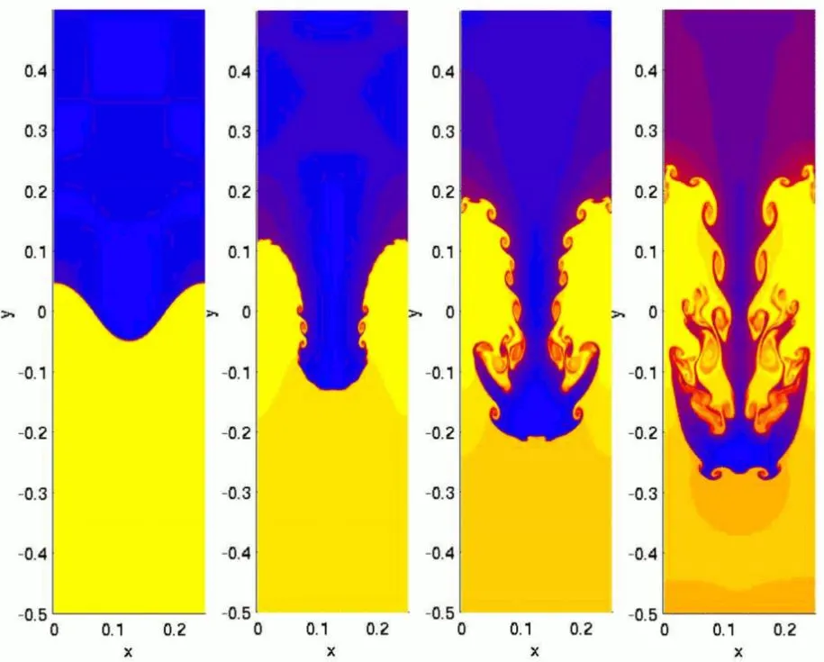
As the Rt instability develops the initial disturbances progress from a linear growth to a non linear growth phase, eventually developing plumes flowing upward and spikes falling downwards. In linear phase the fluid movement can be closely approximated by linear equation, and amplitude of disturbance is growing eponentially with time. In non linear phase disturbances amplitude is much higher than the linear phase and non linear eqautions are needed to determine the fluid motion. In general the density disparity between the fluid determines the structure of the subsequent non-linear RT instability flows.
Some practical CFD models that have been based on the mathematical analysis of Rayleigh Taylor waves:
- Kelvin-Helmholtz instability: Instability occur when there is a velocity shear in a single continuous fluid or where there is a velocity difference across the interface between the fluids. Example include wind blowing over water, the instabilty constant is able to manifest itself through waves on a water surface. The KH instability is not only restricted to water surface but can be seen in clouds and many other natural phenomenon.
The theroy predicts the onset of instability an transition to turbulent flows within fluids of different densities moving at various speeds . Helmholtz studied the dynamics of two fluids with different densities when a small disturbances are created, such a wave was introduced at the boundary connecting the fluids.Kevin-helmholtz instability can be characterized as unstable small scale motion ocurring vertically and laterally. For continuously varying distribution of density and velocity the dynamics of KH instability is described by the Taylor- Goldstein equation and the onset is given by the Richardson number Ri. The layer is unstable for Ri<0.25. Richardson number is a dimensionless number that expresses the ratio of buoyancy term to the flow shear term.These effects are common in cloud layers.
Numerically KH instabilty is computed based on temporal and spatial approach means time and space. In temporal appraoch experimenters considers the flow in a periodic or cyclic box moving at mean speeds. In spatial approach experiment is simulated in a lab with natural inlet and outlet condition i.e convective instability.
- Plateau-Rayleigh instability: The Plateau–Rayleigh instability, explains why and how a falling stream of fluid breaks up into smaller packets with the same volume but less surface area. It is related to the Rayleigh-taylor instability and is part of a greater branch of fluid dynamics concerned with fluid thread breakup. This fluid instability is exploited in the design of a particular type of ink jet technology whereby a jet of liquid is perturbed into a steady stream of droplets
The driving force of the Plateau–Rayleigh instability is that liquids, by virtue of their surface tension, tend to minimize their surface area.The explanation of this instability begins with the existence of tiny perturbations in the stream. These are always present, no matter how smooth the stream is. If the perturbations are resolved into sinusoidal components, we find that some components grow with time, while others decay with time. Among those that grow with time, some grow at faster rates than others. Whether a component decays or grows, and how fast it grows is entirely a function of its wave number (a measure of how many peaks and troughs per unit length) and the radius of the original cylindrical stream.It is found that unstable components (that is, components that grow over time) are only those where the product of the wave number with the initial radius is less than unity. KRo<1. The component that grows the fastest is the one whose wave number satisfies the equation.
- Richtmyer–Meshkov instability (RMI) occurs when two fluids of different density are impulsively accelerated. Normally this is by the passage of a shock wave. The development of the instability begins with small amplitude perturbations which initially grow linearly with time. This is followed by a nonlinear regime with bubbles appearing in the case of a light fluid penetrating a heavy fluid, and with spikes appearing in the case of a heavy fluid penetrating a light fluid. A chaotic regime eventually is reached and the two fluids mix. This instability can be considered the impulsive-acceleration limit of the Rayleigh–Taylor instability.
Explanation for adaptation of mathematical models for CFD calculation:
Models used in CFD calculation of RT instability include diffuse interface model and boussineqs approximation method for the formulation of Naviers stokes equation. These model are pure amalgam of coupled non linear system of equations with initial condition and boundary condition like neumann boundary condition; which basically solves set of PDE like mass conservation equation, energy equation.
Solving and modelling approch:
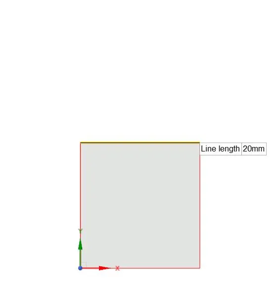
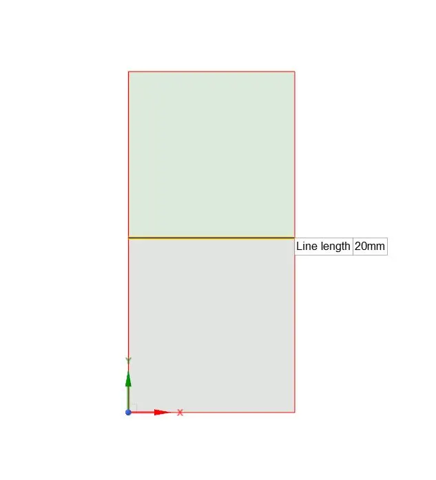
- Create a geometry in spaceclaim with two plane surfaces attached with each of dimension 20mm*20mm
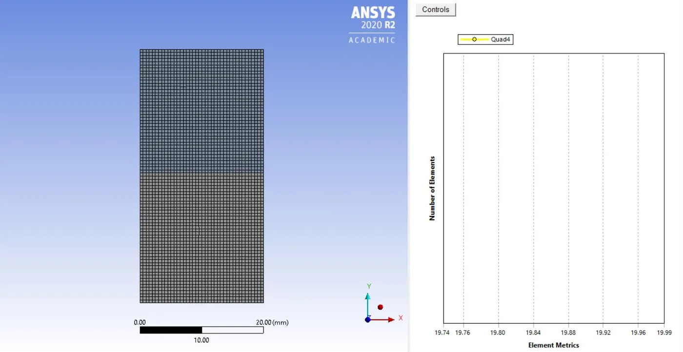
- open the mesh and make a mesh of element size 0.5mm for the baseline mesh
- we run three cases which have a baseline mesh of 0.5mm, 0.25mm and 0.25mm

- setting up physics involves laminar flow with multiphase enabled with water and air as two phases
- Volume of fraction method is enabled and the patches are fixed to 1 for water and 0 for air.
- The contour of volume fraction and animation is setup.
- The results are post processed in CFD post.
Geometry:
spaceclaim model:
we basically take two surfaces i.e one surface on top of another.
-----------------------------------------------------------------------Case 1: Baseline mesh with element size 0.5mm water and air as material--------------------------------------------------------
Case table

Mesh:
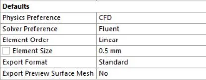

FLUENT setup:
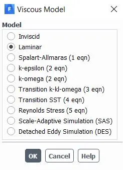
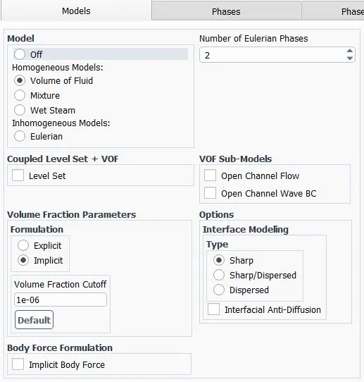
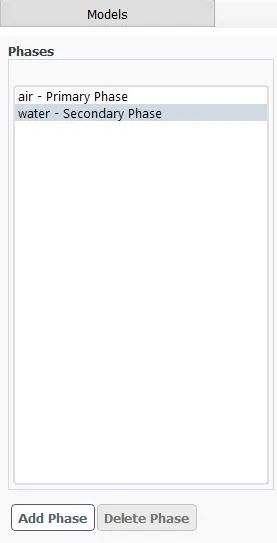
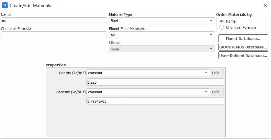
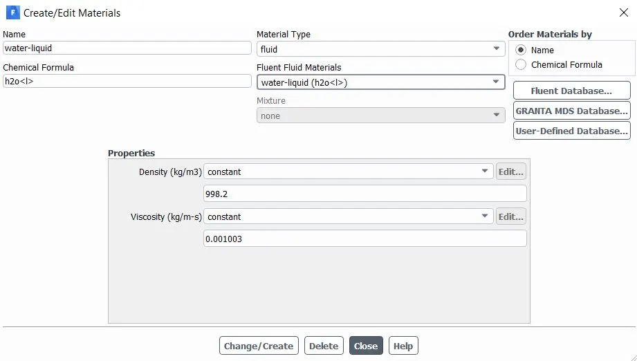
material properties
solver time :
Time step size = 0.025
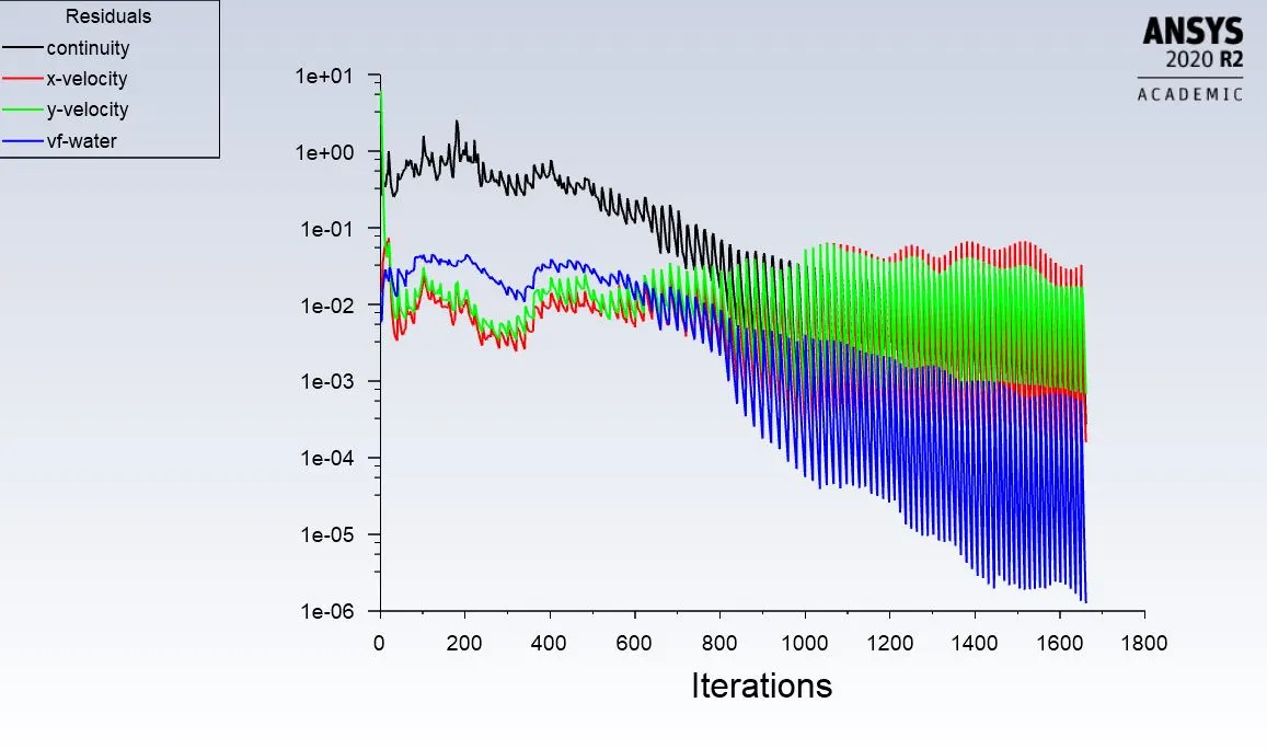
No of iterations = 1660
Residuals:
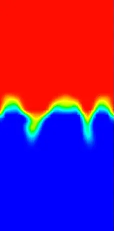
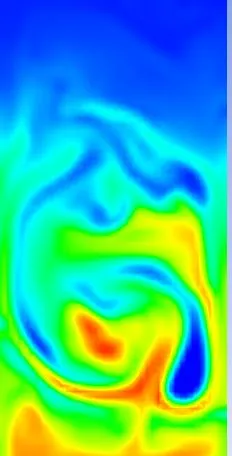
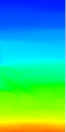
Contours:
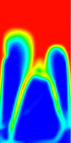
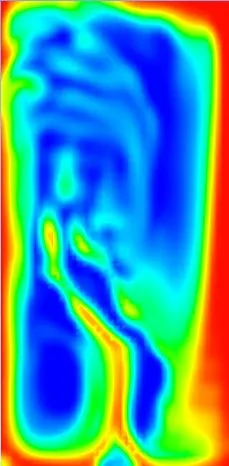
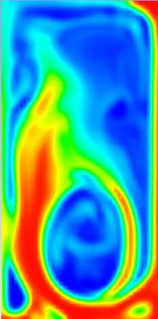
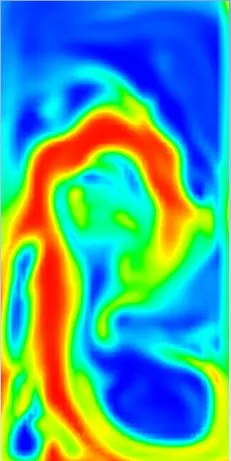
Animation:
--------------------------------------------------------------case 2: refined mesh with element size 0.25mm using air and water as material---------------------------------------------------------
case table:

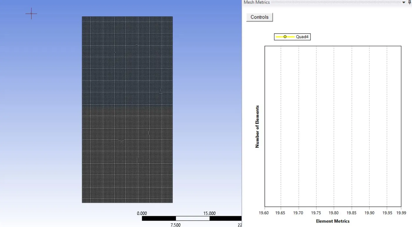
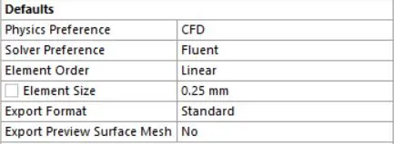
Mesh:

FLUENT setup and Material properties:
Note : The fluent setup and Material properties is same as case1
Solver time:
Time step size = 0.005
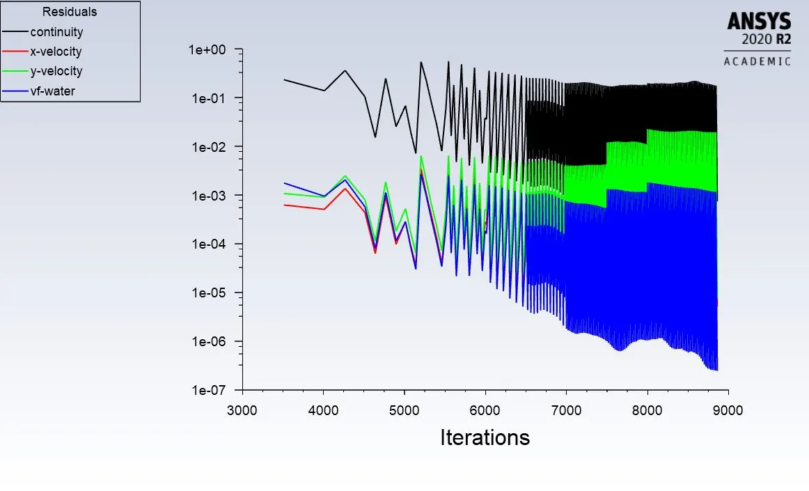
No of iteration = approx 9000
Residuals:
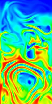
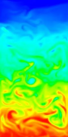
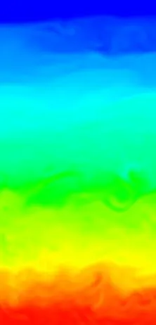
Contours:
Animation:
-----------------------------------------------------------------------------Case 3: refined mesh 0.25mm with water and user defined material-----------------------------------------------------------
case table:

Mesh:
FLUENT setup :
Note : The fluent setup is same as case1
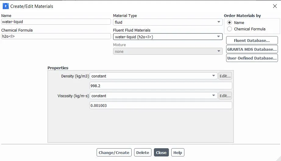
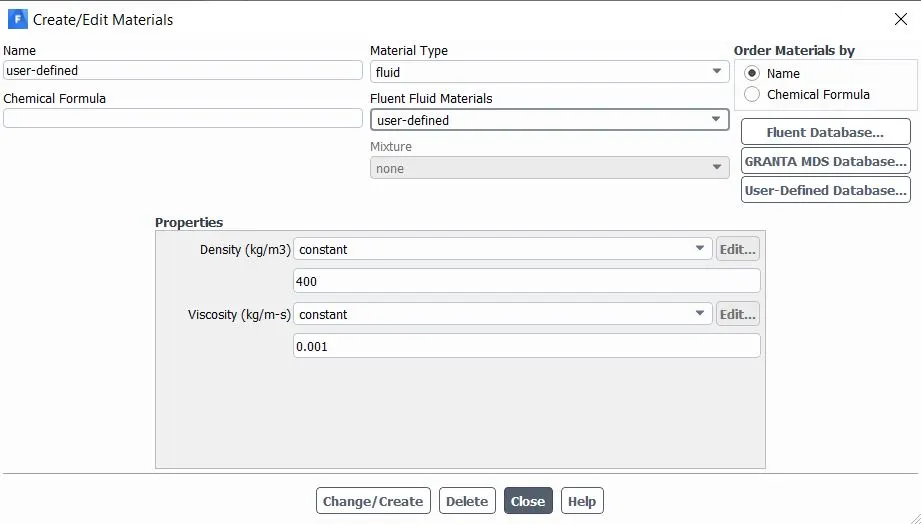
Material properties:
Solver time:
Time step size = 0.005
No of iteration = approx 15600
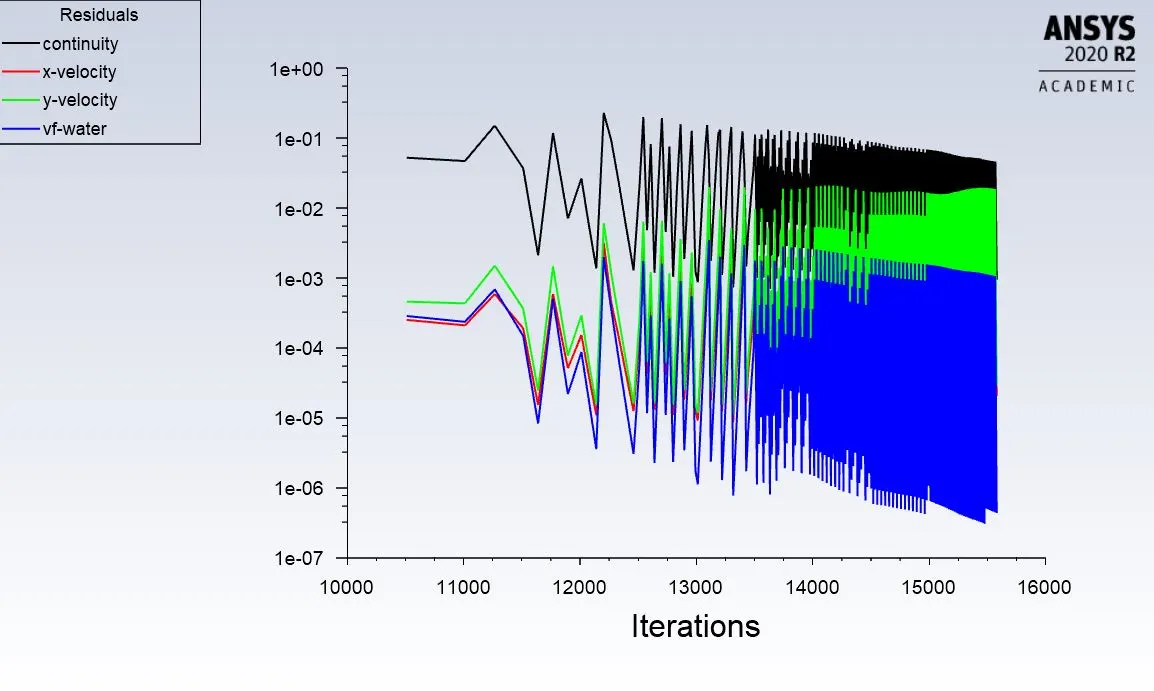
Residuals:
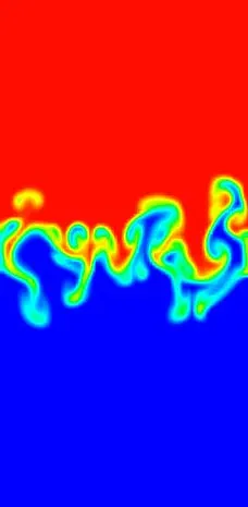
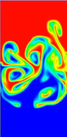
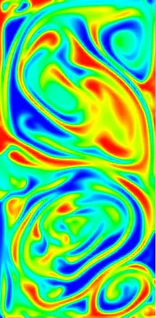
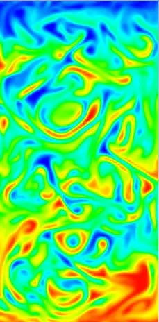
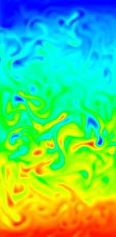
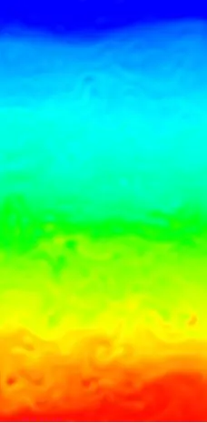
Contours:
Animation:
--------------------------------------------------------------------------------------------------------------------------------------------------------------------------------------
Results:
- RT instability can be seen at the interface of the water and air with excahnge of fluids at the interface.
- The instability can be seen after a few iteration have been run.
- The instabilities are only visualized after the density of top fluids interacts and diffuses in to another.
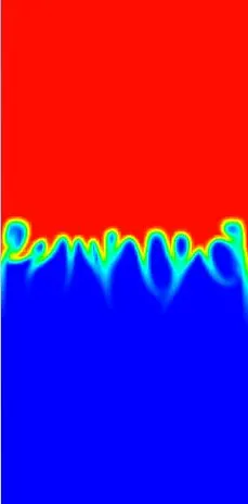
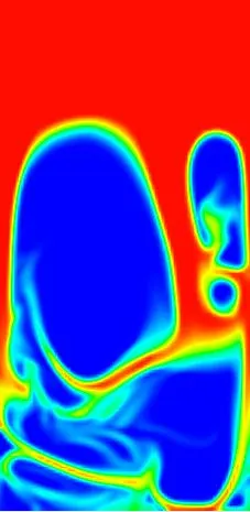
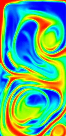
- The instabilities can be better visualized with refined mesh. As we can see that the refined mesh with 0.25mm gives better results.
- Exchange of fluid at interfaces can be divided in to bulk blue zones which are bigger in size and with refined mesh these zones look even more clear.
- The mixing of fluids depends upon the densities and the differences can be seen in case 2 and case3.
why not steady state?
Steady state is used only when we are much concerned with the final outcome of the simulation. whereas transient state is prefered when the ongoing process is more important than the final state result. As in the case of RT instability we are much concerned by the interface mixing and pattern generated which can be only be possible by making a transient state simulation with animation captured with respect to time.
Atwood number and its calculations:
Definition:In fluid dynamics, the Atwood number (A) is a dimensionless-number.The Atwood number is defined as a dimensionless density ratio it is given as:
Formula: `(rho 1-rho2)/(rho1+rho2)`
where `rho1= density -of-heavier -fluid((kg)/m^3)`
`rho2=density-of-lighter-fluid((kg)/m^3)`
Significance
-
The Atwood number is used in the study of Rayleigh Taylor instability.
-
The Rayleigh–Taylor instability, is an instability of an interface between two fluids of different densities, which occurs when the lighter fluid is pushing the heavier fluid.For example, when the water is suspended above oil in the gravity.
-
For Atwood number closer to 1,means the lighter fluid below the heavier fluid takes the form of larger bubble-like plumes.
Calculation:
case 1 and case 2 :
density of heavier fluid (water) `rho1=998.2 (kg)/m^3`
density of lighter fluid (air) `rho2=1.225 (kg)/(m^3)`
Atwood number= `(998.2-1.225)/(998.2+1.225)=0.9975`
case 3:
density of lighter fluid (user-defined) `rho2=400 (kg)/m^3`
density of heavier fluid (water) `rho1=998.2 (kg)/(m^3)`
Atwood number= `(998.2-400)/(998.2+400)=0.43`
we can se in the animation and contours as the atwood number is close to 1 in the case 1 and case 2 the larger plumes are formed and the lighter fluid pushes the heavier fluid.
Conclusions:
- In the three cases we can see the Rayleigh Taylor instability.
- The instabilities can be seen clearer and more accurately with refined mesh sizes.
- The mixing of interfaces and the larger pliumes are seen better for case 2 with refined mesh and Atwood number 0.99, which gives pretty good animation.
- The Atwood number ranges from 0 to 1 and our scenarios lies in between 0.42 to 1.
- According to me the instabilty in case2 and case 3 are better visualized.
- This clearly tells the importance of finer mesh which help us to capture a good amount of physics in transient approach.
References:
https://aip.scitation.org/doi/full/10.1063/1.5100791
https://en.wikipedia.org/wiki/Kelvin%E2%80%93Helmholtz_instability
https://en.wikipedia.org/wiki/Plateau%E2%80%93Rayleigh_instability
https://en.wikipedia.org/wiki/Richtmyer%E2%80%93Meshkov_instability