Challenge

Sensitivity analysis of a combustion reaction with respect to temperature.

AAditya Poojary19 Jan 2021

AIM :

To perform sensitvity analysis on a combustion reaction, and obtain the reactions that are most sensitive to temperature.

Introduction:

A reaction mechanism consists of a number of elementary reactions, which are single step reactions, resulting in the formation of the final products. The pace of an elementary reaction,the reaction rate, is an important factor that influences the product formation. The reaction rate of a reaction is influenced greatly by temperature, among many other factors. However, the vice versa of the previous statement is true. The temperature of the reactants may experience an increase, decrease or no-change, due to the reaction rate, depending on the nature of the reaction. Sensitivity analysis, in this case, can be defined as the change observed in parameters such as temperature, pressure, or species concentration with respect to a certain reaction.

Theory:

There are upwards of two hundred reactions that take place during the combustion of a hydrocarbon such as methane. The GRI-mech 3.0 mechanism (used to perform this combustion simulation), contains a total of three hundred and twenty five reactions. Some reactions do not influence the change in the parameters being observed to a great extent, and obtaining the reaction rates of these reactions are difficult and usually not that important. Some reactions influence the parameters being observed to a greater extent compared to other reactions, and in this case, can be considered as more important reactions. The objective of performing sensitivity analysis, is to obtain these influential reactions. Sifting through the unimportant reactions and obtaining the important reactions, will save computational effort and time by allowing us to gauge the behaviour of set of particular reactions, and how they influence the required parameters. This will also allow us the anticipate the behaviour of the combustion reaction, without wasting computational effort on the other reactions.

Coding Approach:

The following steps were used to perform the sensitivity analysis on the combustion reaction.

Step I: Importing libraries, setting initial conditions.

The sys,NumPy,Cantera and matplotlib libraries were imported into the program. The Cantera library will allow us to simulate the combustion reaction, while NumPy and matplotlib provide superior mathematical support and plotting capabilities, respectively.
The total number of reactions present in the GRI-mech 3.0 mechanism(325 reactions), are set, as well as the total number of sensitive reactions required. The initial temperature is set at 1500K and the initial pressure is set at 1 atm.
The parameter for which the sensitivity analysis is required ,is set by specifying the parameter index. In this case, the required parameter is temperature. This will be elaborated upon in the next step.
The time increment at which the thermodynamic state of the mixture is required is set, as well as the start and end time of the simulation are set.
A few necessary lists are created. A list containing the values between 0 to the total number of reactions required(in this case,325) are specified, and this list will be used to change the reaction over which the sensitivity analysis is being performed, with respect to the required parameter. The 'arange' function is used to achieve this objective.
Lists containing items that are all zeros are created using the 'zeros' function. These lists are created to compile the highest absolute sensitivity coefficient values, the reactions with the highest sensitivity in order of magnitude, all of the highest sensitivity coefficient values, all of the lowest sensitivity values, and the true sensitivity coefficient values(with positive sensitivity coefficient values and negative sensitivity coefficient values), respectively.

Lines of code:

import sys
import numpy as np
import matplotlib.pyplot as plt
import cantera as ct

#Total number of reactions present in the GRI 3.0 mechanism is 325.
n_o_r         = 325
#Top ten most sensitive reactions required:
sen_re        = 10
#Reaction indices
l             = np.arange(0,n_o_r)

#Index of the required parameter:
param_index   = 1

temp          = 1500.0
pres          = ct.one_atm

time_inc      = 5e-6
start_time    = 0
end_time      = 2e-3

#Required lists: 
max_sens      = np.zeros(len(l))
max_sens_true = np.zeros(len(l))
all_min       = np.zeros(sen_re) 
all_max       = np.zeros(sen_re) 
final_list    = np.zeros(sen_re)

Step II: Creating functions.

Three functions are created, and will be elaborated upon individually below.

(A) Function A : Function for sensitivity coefficient:

A 'gas' object is created by using the 'Solution' class of the Cantera library, and the GRI-mech 3.0 mechanism is imported/specified. This class deals with the reactions taking place due to combustion, and the mechanism is optimized for the combustion of fuels. The initial temperature, pressure and mole fractions of the reactant species are defined by using the 'TPX' function of this class. An ideal gas, constant pressure reactor has been chosen for the combustion reaction to be simulated in. The volume will not be held constant, so it can assumed that the constant pressure adiabatic flame temperature will be obtained. The 'IdealGasConstPressureReactor' class has been utilized for this purpose. It takes the gas object as an input argument.
A reactor network is defined by using the 'ReactorNet' class. The instance of the ideal gas constant pressure reactor model defined above is taken as the input argument, and this simulates the reaction over the specified period of time.
A 'for' loop is created, using the total number of reactions as the required range. Within this loop, the reactions for which the sensitivity coefficients are required is specified and imported into the program. This has been done by using the 'add_sensitivity_reaction' function, which uses the range specified in the 'for' loop, as an input argument. This is the only function defined within this 'for' loop.
The absolute and relative tolerances are specified, and are essentially the stopping criteria for the numerical method used to compute the thermodynamic states of the system at a particular time step. Similarly, the absolute and relative tolerances for sensitivity coefficients are specified as well.
A 'for' loop using the range of values between the start and end times of the simulation using the time increment as the step size, is created. The 'arange' function has been used, as it allows the use of float values in the range function.
Within the loop, the 'advance' function is used to integrate the function at the required time increment, and will provide the thermodynamic states of the species at a particular time.
The 'sensitivity' function is utilized to obtain the sensitivity coefficient of a reaction with respect to a certain parameter, and takes two arguments. The 'component_name' function converts the component index provided to a string, and can be displayed in the console if printed. The parameter is mapped to a certain index, and changing this allows us to change the required parameter. In this case, temperature is mapped to component index '1'. The second input argument that the sensitivity function takes, is the reaction itself. The reaction is mapped to a specific index, and the sensitivity of the reaction specified, with respect to the required parameter, will be obtained.
The 'append' function is used to store the thermodynamic states of the mixture at all of the required time steps, and is essentially a data dump. The sensitivity coefficient will be stored using this function as well.
The parameter name and the 'gas' object are defined as global variables.
The initial temperature, pressure, the reaction index, number of reactions,range value for specified list,start and end time, and the time increment are taken as required input arguments for this function.

Lines of code:

#function used to obtain the sensitivity with respect to the required parameter, over the specified range of time steps.
def sensitivity_(temp,pres,l,n_o_r,range_val,param_index,start_time,end_time,time_inc):
	global gas, parameter

	gas     = ct.Solution('gri30.xml')
	gas.TPX = temp, pres, 'CH4:1, O2:2, N2:7.52'
	r       = ct.IdealGasConstPressureReactor(gas, name='R1')
	sim     = ct.ReactorNet([r])

	for i in range(n_o_r):
		r.add_sensitivity_reaction(i)
		

	sim.rtol             = 1.0e-6
	sim.atol             = 1.0e-15
	sim.rtol_sensitivity = 1.0e-6
	sim.atol_sensitivity = 1.0e-6

	states    = ct.SolutionArray(gas,extra = ['t','sens'])

	for t in np.arange(start_time,end_time,time_inc):
		sim.advance(t)
		sens  = sim.sensitivity(r.component_name(param_index),l[range_val-1])
		states.append(r.thermo.state,t = t,sens = sens)

	parameter = r.component_name(param_index)

	return states

(B) Function B : Function for list subtraction:

The use of this function will be elaborated upon in the in the next section.

An empty list is created, and will contain the result of the subtraction of the two lists.
The 'zip' function is used, taking the lists that are to be subtracted, as input arguments. Doing this will ensure that the items with the same index will be operated upon.
A 'for' loop is created, and the two required lists are subtracted. The result of the list is appended to the empty list mentioned above, and the 'append' function is used for this purpose. In this case, the lists 'max_sens_true' is subtracted by 'max_sens', and these two lists are the required input arguments for this function.
The logic behind this will be explained in the next section.
This function is set to return the difference of the two lists.

Lines of code:

#function used to subtract lists:
def list_subtraction(max_sens,max_sens_true):
	sol  = []
	sub  = zip(max_sens,max_sens_true)

	for max_sens_i,max_sens_true_i in sub:
		sol.append(max_sens_i - max_sens_true_i)

	new  = sol

	return new

(C) Function C : Function used to obtain the indices of the required number of reactions with the highest sensitivity coefficient values:

A list consisting of zeroes as items, is created using the 'zeros' function, and the length of the list is the total number of high sensitivity reactions required. This list will store the indices of the reactions with the highest sensitivity coefficient values, in order of magnitude('in_order').
A 'while' loop is created, and the stopping criterion is set as the total number of sensitive reactions required..
Inside the loop, a couple of maneuvers are taking place. As mentioned above, two lists 'max_sens' and 'max_sens_true' have been created. The list 'max_sens', will contain all of the maximum sensitivity coefficient values of each reaction with respect to the required parameter. The 'max_sens_true' list, will contain the highest value of the maximum sensitivity coefficient values present in the 'max_sens' list, while the rest of the items in the list are zeroes. Another important point to note is that the position or index of the highest value of the maximum sensitivity coefficient values in the 'max_sens' list, will be the same as the 'max_sens_true' list.
The highest value of the max sensitivity values in the 'max_sens' list is obtained using the 'max' function, and it's index is found using the 'argmax' function, and both of these functions are used to place the highest value present in the 'max_sens' list in the same position, in the 'max_sens_true' list. To reiterate this point, the index of item containing the highest sensitivity value in the 'max_sens' list, will be identical to the 'max_sens_true' list.
After this has been done, the 'max_sens_true' list is subtracted from the 'max_sens' list using the function for list subtraction mentioned above. Doing this will only reduce the the highest value in the 'max_sens' list to zero, while keeping the rest of the items in the list intact. The new 'max_sens' list, is taken as the result of this subtraction. Doing this will allow us to obtain the second highest sensitivity coefficient value present in the 'max_sens' list. At the end of the loop, the 'max_sens_true' list is defined as a list of zeroes again, in order to avoid errors in the maximum value computation.
The loop will continue until the total number of sensitive reactions required are obtained, and the loop performs this iteratively.
This function is set to return a list of the indices of the sensitive reactions, from highest to the lowest maximum sensitivity.
The function takes 'max_sens','max_sens_true' and the number of sensitive reactions('sen_re') required as input arguments.

Lines of code:

#Function used to find the reactions with the highest values of sensitivity:
def max_sensitivity(max_sens,max_sens_true,sen_re):
	it = 0
	i  = 0
	in_order = np.zeros(sen_re)
	while it < (sen_re):

		max_sens_true[np.argmax(max_sens)] = max(max_sens)
		in_order[i]    = np.argmax(max_sens)
		iter_sens      = list_subtraction(max_sens,max_sens_true)

		max_sens       = iter_sens
		it             = it + 1
		i              = i  + 1

		max_sens_true = np.zeros(len(l))

	return in_order

Step III: Obtaining sensitivity coefficient values,maximum sensitivity coefficient values and their respective reactions.

A 'for' loop is created, using the total number of reactions as the required range.
Within the loop,Function A is used to calculate the sensitivity values for all of the reactions with respect to the defined parameter, over all of the time steps('sens_all').
The maximum absolute value of sensitivity coefficient for each reaction is compiled into the 'max_sens' list, by using the 'max' and 'abs' functions.
Coming out of the loop, the reactions with the highest sensitivity coefficient values are obtained by running Function C, taking the newly created list 'max_sens' as an input argument, as well as the other two required argument('max_sens_true' and 'sen_re'). They have been stored in the list defined as 're_max_sen' and 're_sen_all'. The difference between the two lists is the fact that 're_sen_all' takes the total number of reactions(325 reactions), as the third input argument, and will contain the indices of the reactions in order of greatest sensitivity to the least sensitivity.
Another 'for' loop is created, except this time, it utilizes the newly created list of values as the range. This new list, containing the indices of the reactions with the highest sensitivity, are inserted into Function A, and their senstivities are obtained.
The high sensitivity reaction strings associated with the indices compiled in the list mentioned above, can be obtained by using the 'reaction_equations' function of the 'Solution' class. The function takes the index associated with the reaction, and can be printed in the console using the print command.
The maximum and minimum values of sensitivity coefficients present in each of the high sensitivity reactions are compiled into lists('all_min' and 'all_max').
An 'if-else' loop is created inside this loop. If the absolute value of the item in the 'all_min' list is greater than the absolute value of the item in the 'all_max' list(both items have the same index), the 'all_min' value will be added to the final list. If this condition is not true, the 'all_max' value will be added to the final list. The final list contains the sensitivity coefficient values of the reactions with the highest sensitivity, and will include negative and positive sensitivity values, unlike any of the previous lists mentioned above. This list will be used for displaying the values in the console and will be used for plotting purposes.
A final 'for' loop is created, using the total number of reactions as the required range. This is used to print all of the reactions in order of sensitivity.
The following printing commands were used in this section.

Plotting commands:

figure : Used to assign the figure number.
title : Used to provide a title to the plot.
plot : Used to create a simple line plot. The sensitivity coefficient(with respect to the temperature) vs time is plotted using this function. The 'label' argument is used to create a label for the plot to be used in the legend.
xlabel,ylabel: Used to name the X and Y axes respectively.
legend : Creates the legend for the plot.
show : Displays the plot.

Lines of code:

#Obtaining the sensitivity values of the reactions displaying the highest sensitivity:
for k in range(1,len(re_max_sen)):
	imp_final       = sensitivity_(temp,pres,re_max_sen,n_o_r,k,param_index,start_time,end_time,time_inc)
	reactions       = gas.reaction_equations([re_max_sen[k-1]])
	all_min[k-1]    = np.min(imp_final.sens)
	all_max[k-1]    = np.max(imp_final.sens)

	print('Reaction '+ str(int(re_max_sen[k-1]))+': ' + str(reactions))
	
	if ((abs(all_min[k-1]))>(abs(all_max[k-1]))):
		final_list[k-1] = all_min[k-1]
		print('Max sensitivity coefficient value(with respect to',str(parameter),'): ',final_list[k-1])
	else:
		final_list[k-1] = all_max[k-1]
		print('Max sensitivity coefficient value(with respect to',str(parameter),'): ',final_list[k-1])
	print('n')

	plt.figure(1)
	plt.title('Sensitivity coefficient vs simulation time(s)')
	plt.plot(imp_final.t,imp_final.sens,label= 'Reaction '+ str(int(re_max_sen[k-1])))
	plt.xlabel('Time(s)')
	plt.ylabel('Sensitivity coefficient')
	plt.legend()

print('Reactions in order of greatest sensitivity to least sensitivity(all reactions):')

for f in range(1,len(l)):
	react_str_1  = gas.reaction_equations([re_sen_all[f-1]])
	print('Reaction '+ str(int(re_sen_all[f-1]))+': ' + str(react_str_1))

Step IV: Bar graph plotting

A 'for' loop is created, using the length of the total number sensitive reactions required as the required range.
The required reaction strings are defined using the same 'reaction_equations' command. These strings will be used in the bar graph.
The sensitivity results have been normalized to a range between -1 to +1. The formula for normalization has been defined within the loop, and uses the values in the final list. These normalized values are then plotted against their respective reactions in a bar graph. A bar graph for the non-normalized sensitivity values has been created as well, using the values from the final list without any conversion.

Plotting commands:

figure : Used to assign the figure number.
title : Used to provide a title to the plot.
barh : Used to create a horizontal bar graph. The reactions vs maximum sensitivity coefficient with respect to the temperature(normalized and non-normalized) bar plot is created using this function.
xlabel,ylabel : Used to name the X and Y axes respectively.
show : Displays the plot.

Lines of code:

for q in range(1,len(re_max_sen)):
	react_str_2 = gas.reaction_equations([re_max_sen[q-1]])

	plt.figure(2)
	plt.xticks(np.arange(-1.1,1.1,0.1))
	plt.xlabel('Sensitivity coefficient')
	plt.ylabel('Reactions coefficient')
	plt.title('Sensitivity vs Reactions(Normalized)')
	width      = 1

	normalized = (2.*((final_list[q-1] - np.min(final_list))/np.ptp(final_list)))-1

	plt.barh(str(react_str_2),normalized,width)

	plt.figure(3)
	plt.xlabel('Sensitivity coefficient')
	plt.ylabel('Reactions')
	plt.title('Sensitivity coefficient vs Reactions')

	plt.barh(str(react_str_2),final_list[q-1])

plt.show()

CODE:

The following code was used to obtain the results.

*Note: The following code takes around 1 hour 45 minutes to 2 hours(depending on computer specifications) to obtain the results, due to the volume of the reactions considered.

import sys
import numpy as np
import matplotlib.pyplot as plt
import cantera as ct

#Total number of reactions present in the GRI 3.0 mechanism is 325.
n_o_r         = 325
#Top ten most sensitive reactions required:
sen_re        = 10

#Reaction indices
l             = np.arange(0,n_o_r)

#Index of the required parameter:
param_index   = 1

temp          = 1500
pres          = ct.one_atm

time_inc      = 5e-6
start_time    = 0
end_time      = 2e-3

#Required lists: 
max_sens      = np.zeros(len(l))
max_sens_true = np.zeros(len(l))
all_min       = np.zeros(sen_re) 
all_max       = np.zeros(sen_re) 
final_list    = np.zeros(sen_re) 

#function used to obtain the sensitivity with respect to the required parameter, over the specified range of time steps.
def sensitivity_(temp,pres,l,n_o_r,range_val,param_index,start_time,end_time,time_inc):
	global gas, parameter

	gas     = ct.Solution('gri30.xml')
	gas.TPX = temp, pres, 'CH4:1, O2:2, N2:7.52'
	r       = ct.IdealGasConstPressureReactor(gas, name='R1')
	sim     = ct.ReactorNet([r])

	for i in range(n_o_r):
		r.add_sensitivity_reaction(i)
		

	sim.rtol             = 1.0e-6
	sim.atol             = 1.0e-15
	sim.rtol_sensitivity = 1.0e-6
	sim.atol_sensitivity = 1.0e-6

	states    = ct.SolutionArray(gas,extra = ['t','sens'])

	for t in np.arange(start_time,end_time,time_inc):
		sim.advance(t)
		sens  = sim.sensitivity(r.component_name(param_index),l[range_val-1])
		states.append(r.thermo.state,t = t,sens = sens)

	parameter = r.component_name(param_index)

	return states

#function used to subtract lists:
def list_subtraction(max_sens,max_sens_true):
	sol  = []
	sub  = zip(max_sens,max_sens_true)

	for max_sens_i,max_sens_true_i in sub:
		sol.append(max_sens_i - max_sens_true_i)

	new  = sol

	return new

#Function used to find the reactions with the highest values of sensitivity:
def max_sensitivity(max_sens,max_sens_true,sen_re):
	it = 0
	i  = 0
	in_order = np.zeros(sen_re)
	while it < (sen_re):

		max_sens_true[np.argmax(max_sens)] = max(max_sens)
		in_order[i]    = np.argmax(max_sens)
		iter_sens      = list_subtraction(max_sens,max_sens_true)

		max_sens       = iter_sens
		it             = it + 1
		i              = i  + 1

		max_sens_true = np.zeros(len(l))

	return in_order

#Obtaining the sensitivity values for all reactions:
for j in range(1,len(l)):
	sens_all        = sensitivity_(temp,pres,l,n_o_r,j,param_index,start_time,end_time,time_inc)
	max_sens[j-1]   = max(abs(sens_all.sens))



print('Parameter used: ',parameter,'n')

#List containing the indices of the reactions with the highest sensitivity, in order of magnitude:
re_max_sen          = max_sensitivity(max_sens,max_sens_true,sen_re)
re_sen_all          = max_sensitivity(max_sens,max_sens_true,n_o_r )

print('Indices of the reactions with maximum sensitivity(according to magnitude of sensitivity):')
print(re_max_sen,'n')

print('Reactions in order of greatest sensitivity to least sensitivity(reactions with the highest sensitivity coefficient):','n')

#Obtaining the sensitivity values of the reactions displaying the highest sensitivity:
for k in range(1,len(re_max_sen)):
	imp_final       = sensitivity_(temp,pres,re_max_sen,n_o_r,k,param_index,start_time,end_time,time_inc)
	reactions       = gas.reaction_equations([re_max_sen[k-1]])
	all_min[k-1]    = np.min(imp_final.sens)
	all_max[k-1]    = np.max(imp_final.sens)

	print('Reaction '+ str(int(re_max_sen[k-1]))+': ' + str(reactions))
	
	if ((abs(all_min[k-1]))>(abs(all_max[k-1]))):
		final_list[k-1] = all_min[k-1]
		print('Max sensitivity coefficient value(with respect to',str(parameter),'): ',final_list[k-1])
	else:
		final_list[k-1] = all_max[k-1]
		print('Max sensitivity coefficient value(with respect to',str(parameter),'): ',final_list[k-1])
	print('n')

	plt.figure(1)
	plt.title('Sensitivity coefficient vs simulation time(s)')
	plt.plot(imp_final.t,imp_final.sens,label= 'Reaction '+ str(int(re_max_sen[k-1])))
	plt.xlabel('Time(s)')
	plt.ylabel('Sensitivity coefficient')
	plt.legend()

print('Reactions in order of greatest sensitivity to least sensitivity(all reactions):')

for f in range(1,len(l)):
	react_str_1  = gas.reaction_equations([re_sen_all[f-1]])
	print('Reaction '+ str(int(re_sen_all[f-1]))+': ' + str(react_str_1))

for q in range(1,len(re_max_sen)):
	react_str_2 = gas.reaction_equations([re_max_sen[q-1]])

	plt.figure(2)
	plt.xticks(np.arange(-1.1,1.1,0.1))
	plt.xlabel('Sensitivity coefficient')
	plt.ylabel('Reactions coefficient')
	plt.title('Sensitivity vs Reactions(Normalized)')
	width      = 1

	normalized = (2.*((final_list[q-1] - np.min(final_list))/np.ptp(final_list)))-1

	plt.barh(str(react_str_2),normalized,width)

	plt.figure(3)
	plt.xlabel('Sensitivity coefficient')
	plt.ylabel('Reactions')
	plt.title('Sensitivity coefficient vs Reactions')

	plt.barh(str(react_str_2),final_list[q-1])

plt.show()

Results:

The following image displays the results obtained in the Python console.

Fig(a) Console display.

The results displayed above will be elaborated upon with the graphs displayed below.

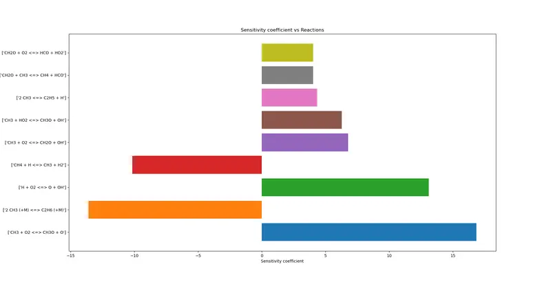
Fig(b) Bar graph for sensitivity coefficient vs reactions.

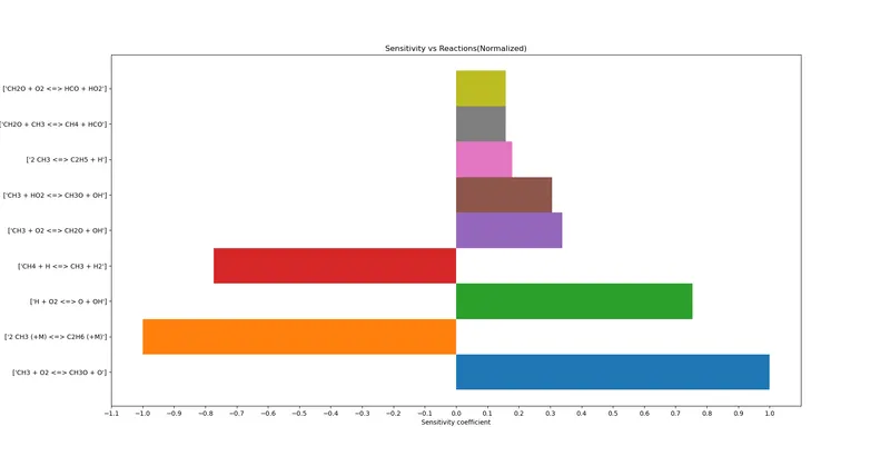
Fig(c) Bar graph for sensitivity coefficient vs reactions[normalized].

From the graphs displayed above, it can be observed that the results obtained are fairly logical. The significance of the most sensitive reactions will be elaborated upon below:

(1) `CH_3 + O_2 <=> CH_3O + O`

Observing the bar graph displayed above, it can be seen that the sensitvity coefficient of the reaction is positive in nature. The reason behind this is the nature of the reaction itself. This reaction is a chain-branching reaction, and promotes the production of free radicals. Free radicals contribute greatly to combustion, and the free radical production influences the pace of the combustion reaction. In this case, it can be observed that methoxy is produced, which is a radical in nature. This suggests that this reaction contributes to temperature increase in the system. This essentially means that this reaction propogates the generation of more free radicals, and free radicals themselves react with other species to form more free radicals.

(2) `2 CH_3 (+M) <=> C_2H_6 (+M)`

Observing the bar graph above, it can be seen that the sensitivity coefficient of this reaction is negative in nature. The reason behind this is the fact that this reaction counters the reaction mentioned above, in terms of result. It can be seen that there are two methyl radicals in this reaction. As mentioned above, the production of radicals is beneficial to combustion, and in consequence, the temperature increase of the system. However in this case, the two methyl radicals react with each other, and form ethane. Ethane is a stable compound, and the free radicals consumed by this reaction prevent the creation of more free radicals. This reaction is a chain-termination reaction, and will occur at the end of the reaction when the free radicals begin reducing in concentration. The occurence of this reaction during the combustion period is detrimental to combustion and consequently, the temperature increase in the system.

(3) `H + O_2 <=> O + OH`

The benefit of this reaction on combustion is very apparent, as the production of hydroxyl radicals contributes to the increase in the radical concentration, and hence increases the temperature of the system. This reaction is a chain-branching reaction as well, and is regarded as an important reaction when the combustion of hydrocarbons is concerned.

(4) `CH_4 + H <=> CH_3 + H_2`

Observing the bar graph, the sensitivity of this reaction is negative in nature. At first glance, this reaction seems to go against what has been established above. It can be seen that a methoxy radical is produced from the reaction, and logically, should contribute to the increase of the temperature of the system. However, the production of hydrogen is not desirable in this case. Ideally, the hydrogen should form water upon reacting with the oxygen. Hence, it can be said that the production of unreacted hydrogen in this reaction will be detrimental to temperature increase in the system.

Upon observing the other positive high sensitivity reactions in the bar graph, it is clear that the generation of radicals is a common trend among these reactions, and have a positive effect on the temperature increase.

The console display shown in Fig(a), displays the reactions with the highest values of sensitivity, and the order of the reactions from greatest sensitivity to least sensitivity.

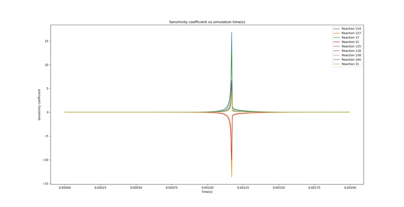
Fig(d) Sensitivity coefficient vs time period.

Observing the plot above, it can be seen that all of the highest sensitivity values are obtained at around the same time step. The time at which this occurs is the auto-ignition delay time.

Sensitivity analysis of a combustion reaction with respect to temperature.

Ship work like this
in your own course.

Talk to a career counsellor

Ship work like thisin your own course.

Talk to a career counsellor

Ship work like this
in your own course.