Reaction mechanism reduction of a combustion reaction.
Aim: To create a reduced reaction mechanism for methane combustion, for different initial conditions of temperature, pressure, and equivalence ratio.
Introduction:
A reaction mechanism consists of a number of elementary reactions, which are single-step reactions, resulting in the formation of the final products. The pace of an elementary reaction, the reaction rate, is an important factor that influences the product formation. The reaction rate of a reaction is influenced greatly by temperature, among many other factors. However, the vice versa of the previous statement is true. The temperature of the reactants may experience an increase, decrease, or no-change, due to the reaction rate, depending on the nature of the reaction. Sensitivity analysis, in this case, can be defined as the change observed in parameters such as temperature, pressure, or species concentration with respect to a certain reaction. Performing sensitivity analysis allows us to identify vital reactions, and manipulate the pace at which the reaction takes place by understanding the behaviour of these particular elementary reactions.
Theory:
The G.R.I 3.0 mechanism is a reaction mechanism set that is able to simulate the combustion of natural gases, and in this case, methane-air combustion. This reaction mechanism contains three hundred and twenty-five elementary reactions in total. Each reaction is associated with a reaction rate, and this is included in the file. However, there are multiple species, reactions, gas types, and species transport equations involved as well. When the combustion of gas takes place, there are a number of elementary reactions that influence quantities such as temperature, pressure, and reaction rate to a greater degree, compared to other reactions. The objective of performing sensitivity analysis is to obtain these influential reactions. Sifting through the unimportant reactions and obtaining the important reactions, will save computational effort and time by allowing us to gauge the behaviour of a set of particular reactions, and how they influence certain parameters. However, this is not the only use of performing sensitivity analysis. Once sensitivity analysis is performed, it is possible to order the reactions with respect to sensitivity towards a certain parameter, and then compile these reactions into their own mechanism files. The total number of reactions that are involved in the combustion of a specific gas will be reduced significantly, and this will yield results that are nearly identical to the simulation that uses the entire set of elementary reactions in the G.R.I 3.0 mechanism file. Doing this will reduce the time required for simulating more complex cases.
Coding Approach:
The following steps were used to perform the sensitivity analysis on the combustion reaction.
Step I: Importing libraries, setting initial conditions.
- The os, sys, NumPy, Cantera, heapq, and matplotlib libraries were imported into the program. The Cantera library will allow us to simulate the combustion reaction, while NumPy and matplotlib provide superior mathematical support and plotting capabilities, respectively.
- The heapq library will allow us to sort the reactions with respect to sensitivity and will be explained in the sections that follow.
- The total number of reactions present in the GRI-mech 3.0 mechanism(325 reactions), is set, as well as the total number of sensitive reactions required. The initial temperature, pressure, and equivalence ratios are set as the following values.
| Temperature state values(T) | 950 K, 1050 K, and 1150 K |
| Pressure state values(P) | 3 bar, 4 bar, and 5 bar |
| Equivalence ratio(`phi`) | 0.5, 1 and 1.5 |
- Three lists were created using the 'zeros' function, taking the length of the temperature, pressure, and equivalence ratio state values lists as an argument. However, these values are added by one, so that the 'for' loop considers the last value in the state value lists. This will be explained in the final step.
- The time increment at which the thermodynamic state of the mixture is required, start time, and end time of the simulation are set.
Lines of code:
import os
import cantera as ct
import matplotlib.pyplot as plt
import numpy as np
import os.path
import heapq as hp

T           = [950,1050,1150]
P           = [3*ct.one_atm,4*ct.one_atm,5*ct.one_atm]
er          = [0.5,1,1.5]

LenT         = np.zeros(len(T)+1)
LenP         = np.zeros(len(P)+1)
Lenphi       = np.zeros(len(er)+1)
Step II: Defining functions
Four functions will be defined in this section.
(A) Function I : Function for obtaining max temperature and ignition delay.
- The temperature, pressure, and equivalence ratio is set using the 'TPX' method. A dictionary for mole fractions is created, and within this dictionary, the number of moles of air is kept as a variable. The reason behind this is that the number of moles of air will vary with the equivalence ratio.
- It should also be noted that the 'gas' object has not been initialized within this function, as it will be taken as an input argument.
- The reactor is set as an ideal gas constant pressure reactor using the 'IdealGasConstPressureReactor' class. The number of reactors is set by using the 'ReactorNet' class and uses the reactor object as an input argument.
- An array is created in order to compile the thermodynamic state values at different time steps using the 'SolutionArray' class. Two extra variables are created to capture the time step and the ignition delay values and have been specified within this class using the 'extra' argument.
- A 'for' loop is defined with the required range of time steps. Within this loop, the 'advance' method is used to obtain the thermodynamic state of the reactor at a particular time step, and the 'append' method is used to insert these values into the array specified above.
- The ignition delay is obtained by creating a nested loop, using the 'if' condition. A check condition is specified outside the 'if' loop and is set as zero. The first 'if' loop checks if the value of 'check' is still zero. The second 'if' loop checks if the temperature has exceeded the initial temperature by 400 degrees(auto-ignition temperature). As soon as this condition is met, the loop will become active and capture the time step, which will be the ignition delay time. In this loop, the 'check' value is incremented by one, and the first 'if' condition will not be satisfied for the remaining time steps.
- This function takes temperature, pressure, equivalence ratio, number of moles of air, and the 'gas' object as input arguments.
Lines of code:
def max_temp_ig_delay(T,P,n_a,n_o_r,gas):

	gas.TPX  = T,P,{'CH4' : 1,'O2' : n_a, 'N2' : n_a*3.76 }
	r        = ct.IdealGasConstPressureReactor(gas, name = 'R1')
	sim      = ct.ReactorNet([r])

	states   = ct.SolutionArray(gas,extra = ['t','ig_delay'])
	check    = 0
	ig_delay = 0

	for t in np.arange(0,5,0.00101):
		sim.advance(t)
		if (check == 0):
			if (r.T >= T + 400):
				ig_delay = sim.time
				check    = check + 1
				continue

		states.append(r.thermo.state,t = t,ig_delay = ig_delay)

	return states
(B) Function II : Function used to obtain the sensitivity of a reaction.
- The 'gas' object has been created in this function, and the 'Solution' class has been used to import the 'gri30.xml' file, which contains the GRI 3.0 mechanism file. The initial temperature, pressure, and mole fractions were defined using the same method mentioned in the previous step. The reactor, number of reactors, and the array used to capture the thermodynamic state variables were defined in the same way as well.
- A 'for' loop is created, using the total number of reactions as the required range. Within this loop, the reactions for which the sensitivity coefficients are required is specified and imported into the program. This has been done by using the 'add_sensitivity_reaction' function, which uses the range specified in the 'for' loop, as an input argument. This is the only function defined within this 'for' loop.
- The absolute and relative tolerances are specified and are essentially the stopping criteria for the numerical method used to compute the thermodynamic states of the system at a particular time step. Similarly, the absolute and relative tolerances for sensitivity coefficients are specified as well.
- A 'for' loop using the range of values between the start and end times of the simulation using the time increment as the step size, is created. The 'arange' function has been used, as it allows the use of float values in the range function.
- Within the loop, the 'advance' function is used to integrate the function at the required time increment and will provide the thermodynamic states of the species at a particular time.
- The 'sensitivity' function is utilized to obtain the sensitivity coefficient of a reaction with respect to a certain parameter and takes two arguments. The 'component_name' function converts the component index provided to a string and can be displayed in the console if printed. The parameter is mapped to a certain index, and changing this allows us to change the required parameter. In this case, the temperature is mapped to the component index '1'. The second input argument that the sensitivity function takes, is the reaction itself. The reaction is mapped to a specific index, and the sensitivity of the reaction specified, with respect to the required parameter, will be obtained.
- The 'append' function is used to store the thermodynamic states of the mixture at all of the required time steps and is essentially a data dump. The sensitivity coefficient will be stored using this function as well.
- The parameter name and the 'gas' object are defined as global variables.
- The initial temperature, pressure, the reaction index, number of reactions, range value for the specified list, start and end time, and the time increment is taken as required input arguments for this function.
Lines of code:
#function used to obtain the sensitivity with respect to the required parameter, over the specified range of time steps.
def sensitivity_(temp,pres,l,n_o_r,range_val,param_index,start_time,end_time,time_inc,n_a):


	gas     = ct.Solution('gri30.xml')
	gas.TPX = temp, pres,{'CH4' : 1,'O2' : n_a, 'N2' : n_a*3.76 }
	r       = ct.IdealGasConstPressureReactor(gas, name='R1')
	sim     = ct.ReactorNet([r])

	for x in range(n_o_r):
		r.add_sensitivity_reaction(x)


	sim.rtol             = 1.0e-6
	sim.atol             = 1.0e-15
	sim.rtol_sensitivity = 1.0e-6
	sim.atol_sensitivity = 1.0e-6

	states    = ct.SolutionArray(gas,extra = ['t','sens'])

	for t in np.arange(start_time,end_time,time_inc):
		sim.advance(t)
		sens  = sim.sensitivity(r.component_name(param_index),l[range_val-1])
		states.append(r.thermo.state,t = t,sens = sens)

	return states
(C) Function III : Function used to obtain the reactions that will be used in the reduced reaction mechanism.
- The basic idea behind this function is to use the indices of the most sensitive reactions that have been obtained using Function II. An empty array has been created to store the reaction strings of the high sensitivity reactions.
- A 'for' loop has been defined. The most important part of this function is the range between which the 'for' loop operates. A minimum of 40 sensitive reactions will be considered first. To understand how this function works, the basic gist of the program will be explained in brief.
- The indices of the most sensitive reactions will be compiled into a list. The indices associated with these reactions(in the G.R.I mechanism file), will be used to obtain the reaction string. The first 40 sensitive reactions will be compiled into an array. This reaction set will be injected into a new mechanism file. A new 'gas' object will be created using this mechanism file. The maximum temperature and ignition delay will be calculated using this new 'gas' object. This entire process is done within a loop, and the loop range has been set to 325, which is the total number of reactions in the mechanism file. After the completion of each loop, a sensitive reaction will be added to a new mechanism file and the process will be repeated.
- As mentioned above, a 'for' loop has been created within this function. With each pass of the main loop outside this function, the range of the 'for' loop will be incremented by one. This has been done to increase the number of sensitive reactions that will be added to the reaction array with each pass of the main loop. The sensitive reactions are associated with specific indices in the G.R.I mechanism file, and this will be used to obtain the reaction strings using the 'reactions' function.
- The function is set to return an array of the reactions. The minimum required reactions, the increment value, the list of sensitive reactions, and the object using the 'reactions' function are the input arguments required by the function.
Lines of code:
def reduced_rm(re_max_sen,gas_reactions,min_req_re,reaction_increment):
	reactions           = np.array([])

	for n in np.arange(0,min_req_re+reaction_increment):
		v = re_max_sen[n]
		reactions       = (np.append(reactions,gas_reactions[int(v)]))
	return reactions
(D) Function IV: Main program.
- The total number of reactions present in the GRI-mech 3.0 mechanism(325 reactions), is set, as well as the total number of sensitive reactions required.
- The parameter for which the sensitivity analysis is required is set by specifying the parameter index. In this case, the required parameter is temperature.
- The time increment at which the thermodynamic state of the mixture is required, start time, and end time of the simulation are defined.
- A few necessary lists were created. A list containing the values between 0 to the total number of reactions required(in this case,325) was specified, and this list will be used to change the reaction over which the sensitivity analysis is being performed, with respect to the required parameter. The 'arange' function was used to achieve this objective.
- A list containing items that are all zeros are created using the 'zeros' function. This list has been created to compile the highest absolute sensitivity coefficient values.
- The stoichiometric number of moles of air and fuel are defined. The actual number of moles of fuel is set to '1'. The actual number of moles of air required is computed using the following formula.
`n_a = (n_text(f)*n_text(sa))/(phi*n_text(sf))`
where,
`n_a = text(actual number of moles of air)`
`n_f = text(actual number of moles of fuel)`
`n_text(sa) = text(stoichiometric number of moles of air)`
`n_(text(sf)) = text(stoichiometric number of moles of fuel)`
`phi = text(equivalence ratio)`
- Function I was used to obtain the maximum temperature and ignition delay, and the complete G.R.I mechanism file was used to obtain these values.
- A 'for' loop is created, using the total number of reactions as the required range.
- Within the loop,Function A is used to calculate the sensitivity values for all of the reactions with respect to the defined parameter, over all of the time steps('sens_all').
- The maximum absolute value of the sensitivity coefficient for each reaction is compiled into the 'max_sens' list, by using the 'max' and 'abs' functions.
- The highest sensitivity values in order of magnitude have been obtained using the heapq library. The 'nlargest' function allows us to sort the reactions with respect to highest sensitivity, and the indices associated with these reactions are compiled into a list.
- Five empty arrays have been created using the 'array' function. These arrays will be used to store the total number of reactions that have been considered in a loop, max temperature and ignition delay associated with these reactions, and the reference values of ignition delay and max temperature.
- The minimum number of reactions to be considered in the first loop is set to 40, and the reactions in the G.R.I mechanism file are imported using the 'reactions' method. The variable 'add' in this case is the reaction increment and has been set to 0 initially.
- A 'while' loop was created, and this loop will be active until the total number of reactions in the G.R.I mechanism file(325) has not been reached.
- Function III has been used to obtain the reactions that will be used in the reduced reaction mechanism.
- A new mechanism file has been created using these reactions(gas_red), using the 'Solution' class. The solution class has an input argument known as 'reactions', and the reduced reactions are injected here. All of the species involved have been specified using the 'species' command.
- Function I is used again in order to find the max temperature and ignition delay of the reduced mechanism file.
- All of the values were then appended to the arrays mentioned above using the 'append' function.
- At the end of the loop, the reaction increment is defined again, with an increment of 1.
The following plotting commands have been used to obtain the plots.
(1) Number of reactions vs ignition delay
(2) Number of reaction vs maximum temperature
| figure | Used to assign the figure number and the dimensions of the plot. |
| subplot | Used to define the total number of plots required on one page, and assigning a position to the plot. |
| title | Used to provide a title to the plot. |
| plot | Used to create a line plot. The 'label' is used to provide information pertaining to the nature of the plot, and will be displayed in the legend. |
| xlabel,ylabel | Used to name the X and Y axes respectively. |
| grid | Used to create a grid in the background. |
| show | Displays the plot. |
| legend | Used to create a legend. |
| save_fig | Saves the plot |
Lines of code:
def program(i,j,k,T,P,er):

	gas = ct.Solution('gri30.cti')
	#Total number of reactions present in the GRI 3.0 mechanism is 325.
	n_o_r         = 325
	#Top ten most sensitive reactions required:
	sen_re        = 325
	#Reaction indices
	l             = np.arange(0,n_o_r)

	#Index of the required parameter:
	param_index   = 1

	time_inc      = 5e-4
	start_time    = 0
	end_time      = 5

	#Required lists:
	max_sens      = np.zeros(len(l))

	n_f_s       = 1
	n_a_s       = 2
	n_f         = 1

	temp                = T[i-1]
	pres                = P[j-1]
	phi                 = er[k-1]
	init_val_set        = (temp,pres,phi)
	n_a                 = (n_f*n_a_s)/(phi*n_f_s)

	print(f'Initial values : Temperature : {temp} K, Pressure : {pres} Pa, Equivalence ratio : {phi}')

	A             = max_temp_ig_delay(temp,pres,n_a,n_o_r,gas)
	m_temp        = max(A.T)
	m_id          = max(A.ig_delay)
	print(f'Max temperature = {max(A.T)} K\nIgnition delay  = {max(A.ig_delay)} s \n')

	#Obtaining the sensitivity values for all reactions:
	for z in range(1,len(l)):
		sens_all        = sensitivity_(temp,pres,l,n_o_r,z,param_index,start_time,end_time,time_inc,n_a)
		max_sens[z-1]   = max(abs(sens_all.sens))


	#List containing the indices of the reactions with the highest sensitivity, in order of magnitude:
	re_max_sen          = hp.nlargest(sen_re,range(len(max_sens)),max_sens.__getitem__)

	print('Indices of the reactions with maximum sensitivity(according to magnitude of sensitivity):')
	print(re_max_sen,'\n')

	mt  = ref_igdel = ref_temp  = reduced_temp = reduced_igdel = np.array([])

	gas_reactions= gas.reactions()
	min_req_re   = 40
	add          = 0
	total        = min_req_re+add


	while (total != n_o_r):
		species = gas.species()

		reduced_mech = reduced_rm(re_max_sen,gas_reactions,min_req_re,add)

		gas_red = ct.Solution(thermo='IdealGas',kinetics='GasKinetics',species = species, reactions=tuple(reduced_mech))
		B       = max_temp_ig_delay(temp,pres,n_a,n_o_r,gas_red)

		m_temp1 = np.max(B.T)
		m_id1   = np.max(B.ig_delay)

		total   = min_req_re+add

		print(min_req_re+add)
		print(f'Max temperature = {max(B.T)} K')
		print(f'Ignition delay  = {max(B.ig_delay)} s \n')


		mt  = np.append(mt,(add+min_req_re))
		reduced_igdel = np.append(reduced_igdel,m_id1)
		reduced_temp  = np.append(reduced_temp,m_temp1)
		ref_igdel = np.append(ref_igdel,m_id)
		ref_temp  = np.append(ref_temp,m_temp)

		add   = add + 1

	plt.figure(figsize=(12,8))
	plt.subplot(2,1,1)
	plt.plot(mt,ref_temp,linestyle='--',label = f'Reference Max temperature = {max(B.T)} K')
	plt.plot(mt,reduced_temp,label = f'Max temperature : Reduced mechanism')
	plt.title(f'State values : Temperature = {temp} K, Pressure = {pres} Pa, Equivalence ratio = {phi}')
	plt.xlabel('Number of reactions most sensitive to temperature')
	plt.ylabel('Max temperature(K)')
	plt.legend()

	plt.subplot(2,1,2)
	plt.plot(mt,ref_igdel,linestyle='--',label = f'Reference Ignition delay  = {max(B.ig_delay)} s')
	plt.title(f'State values : Temperature = {temp} K, Pressure = {pres} Pa, Equivalence ratio = {phi}')
	plt.plot(mt,reduced_igdel,label = 'Ignition delay : Reduced mechanism')
	plt.xlabel('Number of reactions most sensitive to temperature')
	plt.ylabel('Ignition delay(s)')
	plt.legend()
	plt.tight_layout()
	plt.savefig(f'State_values_Temperature_{temp}K_Pressure_{pres}Pa_Equivalence ratio_{phi}.png',bbox_inches='tight')
Step III : Final loop
- A nested loop consisting of three 'for' loops have been created. The total number of state values will be used as the range over which the loops will run.
- The outermost 'for' loop is the loop for temperature, the second 'for' loop is for pressure, and the third 'for' loop is for the equivalence ratio. There are 27 potential combinations of state values that can be created out of a `3 times 3` matrix. The first loop will remain active until the two loops within it have completed their runs. This means that for the first state value of temperature, there are 9 potential results with different state values of pressure and equivalence ratio that can be achieved. The equivalence ratio loop is within the pressure loop. So there are three possible combinations that a single state value of pressure can make with 3 different equivalence ratios.
- The loop counter will tell us which set of state values are being computed.
Lines of code:
loop_count  = 0

for i in range(1,len(LenT)):
	for j in range(1,len(LenP)):
		for k in range(1,len(Lenphi)):
			loop_count = loop_count +  1

			print(f'State value set :{loop_count}')
			A = program(i,j,k,T,P,er)

plt.show()
CODE:
import os
import cantera as ct
import matplotlib.pyplot as plt
import numpy as np
import os.path
import heapq as hp

T           = [950,1050,1150]
P           = [3*ct.one_atm,4*ct.one_atm,5*ct.one_atm]
er          = [0.5,1,1.5]

LenT         = np.zeros(len(T)+1)
LenP         = np.zeros(len(P)+1)
Lenphi       = np.zeros(len(er)+1)


def max_temp_ig_delay(T,P,n_a,n_o_r,gas):

	gas.TPX  = T,P,{'CH4' : 1,'O2' : n_a, 'N2' : n_a*3.76 }
	r        = ct.IdealGasConstPressureReactor(gas, name = 'R1')
	sim      = ct.ReactorNet([r])

	states   = ct.SolutionArray(gas,extra = ['t','ig_delay'])
	check    = 0
	ig_delay = 0

	for t in np.arange(0,5,0.00101):
		sim.advance(t)
		if (check == 0):
			if (r.T >= T + 400):
				ig_delay = sim.time
				check    = check + 1
				continue

		states.append(r.thermo.state,t = t,ig_delay = ig_delay)

	return states

#function used to obtain the sensitivity with respect to the required parameter, over the specified range of time steps.
def sensitivity_(temp,pres,l,n_o_r,range_val,param_index,start_time,end_time,time_inc,n_a):


	gas     = ct.Solution('gri30.xml')
	gas.TPX = temp, pres,{'CH4' : 1,'O2' : n_a, 'N2' : n_a*3.76 }
	r       = ct.IdealGasConstPressureReactor(gas, name='R1')
	sim     = ct.ReactorNet([r])

	for x in range(n_o_r):
		r.add_sensitivity_reaction(x)


	sim.rtol             = 1.0e-6
	sim.atol             = 1.0e-15
	sim.rtol_sensitivity = 1.0e-6
	sim.atol_sensitivity = 1.0e-6

	states    = ct.SolutionArray(gas,extra = ['t','sens'])

	for t in np.arange(start_time,end_time,time_inc):
		sim.advance(t)
		sens  = sim.sensitivity(r.component_name(param_index),l[range_val-1])
		states.append(r.thermo.state,t = t,sens = sens)

	return states


def reduced_rm(re_max_sen,gas_reactions,min_req_re,reaction_increment):
	reactions           = np.array([])

	for n in np.arange(0,min_req_re+reaction_increment):
		v = re_max_sen[n]
		reactions       = (np.append(reactions,gas_reactions[int(v)]))
	return reactions


def program(i,j,k,T,P,er):

	gas = ct.Solution('gri30.cti')
	#Total number of reactions present in the GRI 3.0 mechanism is 325.
	n_o_r         = 325
	#Top ten most sensitive reactions required:
	sen_re        = 325
	#Reaction indices
	l             = np.arange(0,n_o_r)

	#Index of the required parameter:
	param_index   = 1

	time_inc      = 5e-4
	start_time    = 0
	end_time      = 5

	#Required lists:
	max_sens      = np.zeros(len(l))

	n_f_s       = 1
	n_a_s       = 2
	n_f         = 1

	temp                = T[i-1]
	pres                = P[j-1]
	phi                 = er[k-1]
	init_val_set        = (temp,pres,phi)
	n_a                 = (n_f*n_a_s)/(phi*n_f_s)

	print(f'Initial values : Temperature : {temp} K, Pressure : {pres} Pa, Equivalence ratio : {phi}')

	A             = max_temp_ig_delay(temp,pres,n_a,n_o_r,gas)
	m_temp        = max(A.T)
	m_id          = max(A.ig_delay)
	print(f'Max temperature = {max(A.T)} K\nIgnition delay  = {max(A.ig_delay)} s \n')

	#Obtaining the sensitivity values for all reactions:
	for z in range(1,len(l)):
		sens_all        = sensitivity_(temp,pres,l,n_o_r,z,param_index,start_time,end_time,time_inc,n_a)
		max_sens[z-1]   = max(abs(sens_all.sens))


	#List containing the indices of the reactions with the highest sensitivity, in order of magnitude:
	re_max_sen          = hp.nlargest(sen_re,range(len(max_sens)),max_sens.__getitem__)

	print('Indices of the reactions with maximum sensitivity(according to magnitude of sensitivity):')
	print(re_max_sen,'\n')

	mt  = ref_igdel = ref_temp  = reduced_temp = reduced_igdel = np.array([])

	gas_reactions= gas.reactions()
	min_req_re   = 40
	add          = 0
	total        = min_req_re+add


	while (total != n_o_r):
		species = gas.species()

		reduced_mech = reduced_rm(re_max_sen,gas_reactions,min_req_re,add)

		gas_red = ct.Solution(thermo='IdealGas',kinetics='GasKinetics',species = species, reactions=tuple(reduced_mech))
		B       = max_temp_ig_delay(temp,pres,n_a,n_o_r,gas_red)

		m_temp1 = np.max(B.T)
		m_id1   = np.max(B.ig_delay)

		total   = min_req_re+add

		print(min_req_re+add)
		print(f'Max temperature = {max(B.T)} K')
		print(f'Ignition delay  = {max(B.ig_delay)} s \n')


		mt  = np.append(mt,(add+min_req_re))
		reduced_igdel = np.append(reduced_igdel,m_id1)
		reduced_temp  = np.append(reduced_temp,m_temp1)
		ref_igdel = np.append(ref_igdel,m_id)
		ref_temp  = np.append(ref_temp,m_temp)

		add   = add + 1

	plt.figure(figsize=(12,8))
	plt.subplot(2,1,1)
	plt.plot(mt,ref_temp,linestyle='--',label = f'Reference Max temperature = {max(B.T)} K')
	plt.plot(mt,reduced_temp,label = f'Max temperature : Reduced mechanism')
	plt.title(f'State values : Temperature = {temp} K, Pressure = {pres} Pa, Equivalence ratio = {phi}')
	plt.xlabel('Number of reactions most sensitive to temperature')
	plt.ylabel('Max temperature(K)')
	plt.legend()

	plt.subplot(2,1,2)
	plt.plot(mt,ref_igdel,linestyle='--',label = f'Reference Ignition delay  = {max(B.ig_delay)} s')
	plt.title(f'State values : Temperature = {temp} K, Pressure = {pres} Pa, Equivalence ratio = {phi}')
	plt.plot(mt,reduced_igdel,label = 'Ignition delay : Reduced mechanism')
	plt.xlabel('Number of reactions most sensitive to temperature')
	plt.ylabel('Ignition delay(s)')
	plt.legend()
	plt.tight_layout()
	plt.savefig(f'State_values_Temperature_{temp}K_Pressure_{pres}Pa_Equivalence ratio_{phi}.png',bbox_inches='tight')


loop_count  = 0

for i in range(1,len(LenT)):
	for j in range(1,len(LenP)):
		for k in range(1,len(Lenphi)):
			loop_count = loop_count +  1

			print(f'State value set :{loop_count}')
			A = program(i,j,k,T,P,er)


plt.show()
Results:
| `T = 950 K` | ||
| `phi = 0.5` | `phi = 1` | |
| `P = text(3 atm)` | 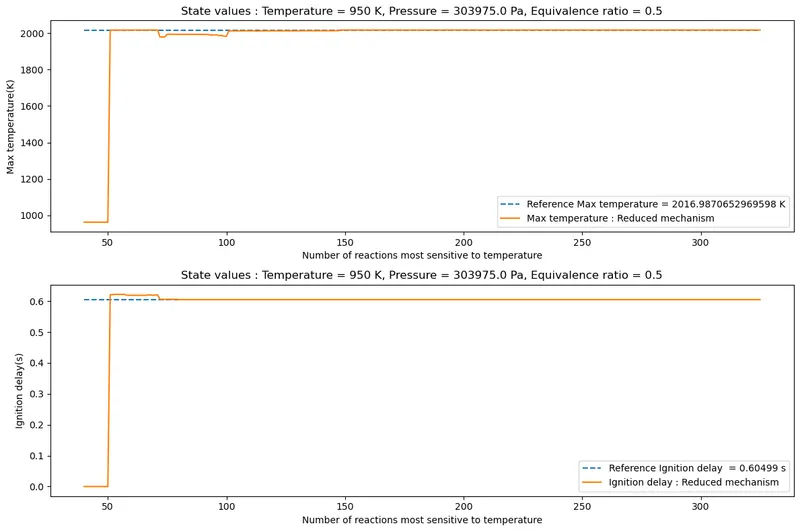 |
 |
| `phi = 1.5` | ||
 |
||
| `P = text(4 atm)` | `phi = 0.5` | `phi = 1` |
 |
 |
|
| `phi = 1.5` | ||
 |
||
| `P = text(5 atm)` | `phi = 0.5` | `phi = 1` |
 |
 |
|
| `phi = 1.5` | ||
 |
||
| `T = 1050 K` | ||
| `phi = 0.5` | `phi = 1` | |
| `P = text(3 atm)` | 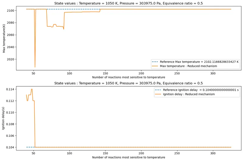 |
 |
| `phi = 1.5` | ||
 |
||
| `P = text(4 atm)` | `phi = 0.5` | `phi = 1` |
 |
 |
|
| `phi = 1.5` | ||
 |
||
| `P = text(5 atm)` | `phi = 0.5` | `phi = 1` |
 |
 |
|
| `phi = 1.5` | ||
 |
||
| `T = 1150 K` | ||
| `P = text(3 atm)` | `phi = 0.5` | `phi = 1` |
 |
 |
|
| `phi = 1.5` | ||
 |
||
| `P = text(4 atm)` | `phi = 0.5` | `phi = 1` |
 |
 |
|
| `phi = 1.5` | ||
 |
||
| `P = text(5 atm)` | `phi = 0.5` | `phi = 1` |
 |
 |
|
| `phi = 1.5` | ||
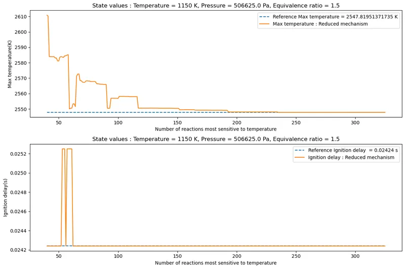 |
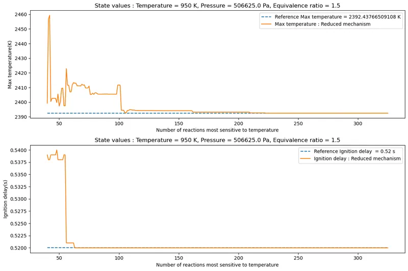
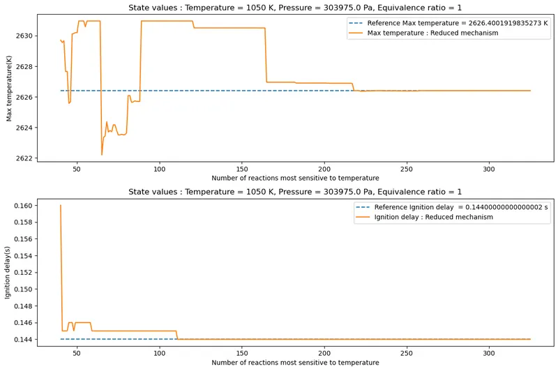
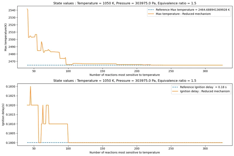
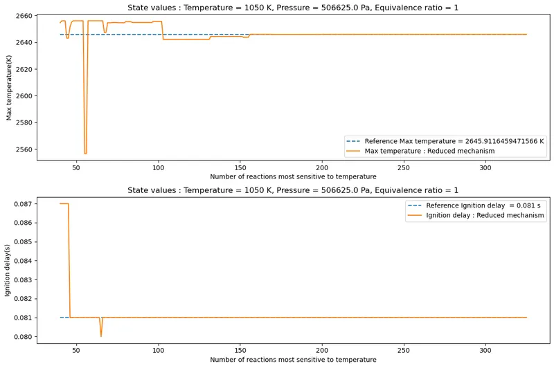
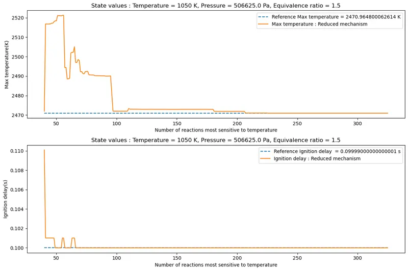
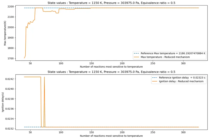
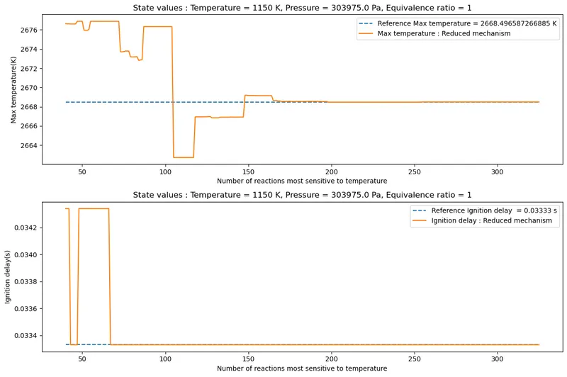
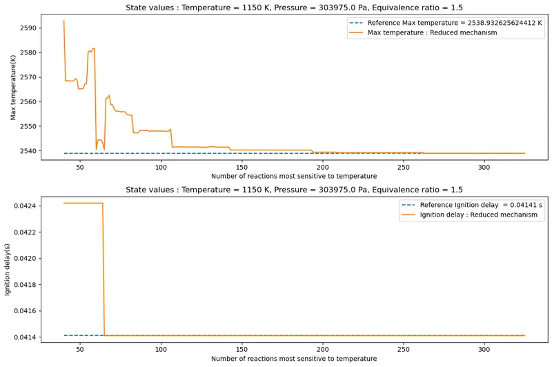
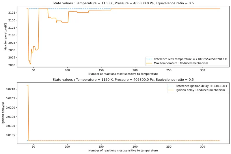
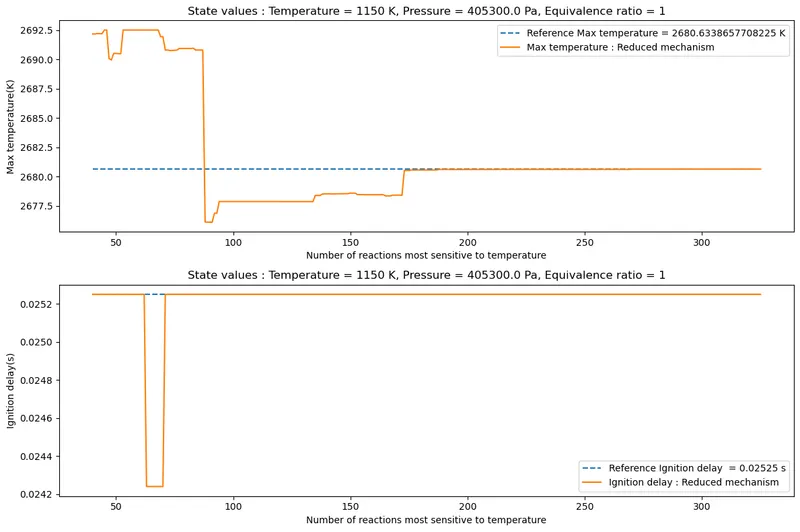
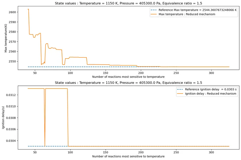
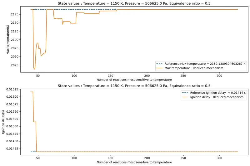
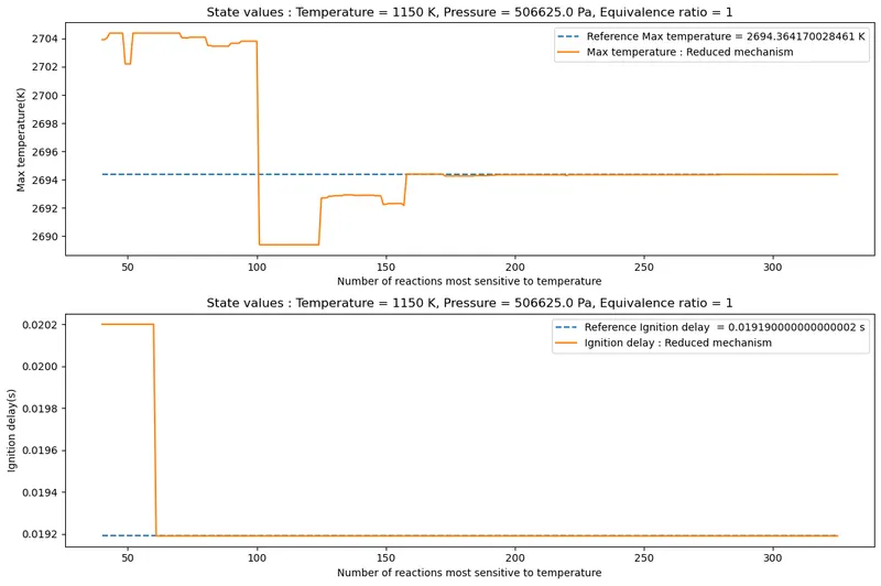
A few inferences can be drawn from the plots displayed above. In order to discuss the unique behaviour of the fuel under various conditions, this discussion will be divided according to the type of fuel mixture.
Rich mixtures:
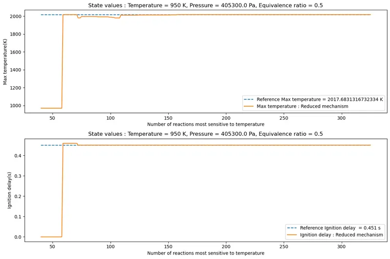
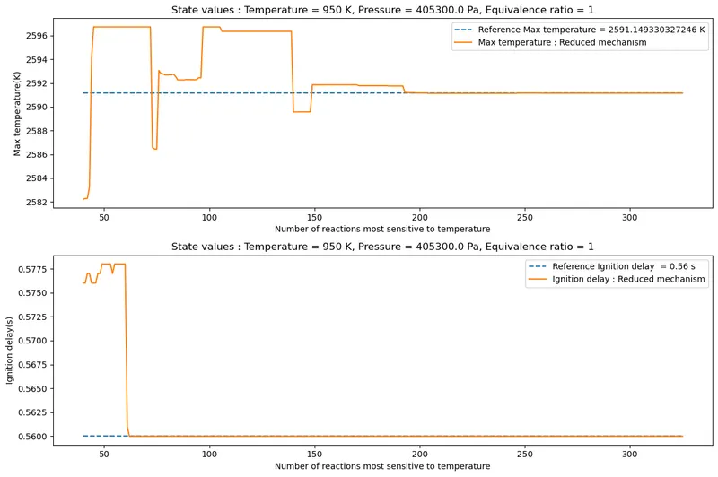
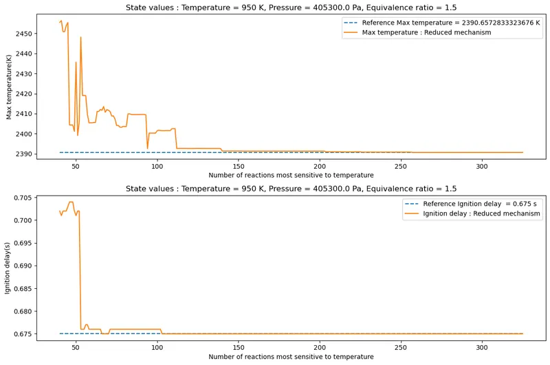
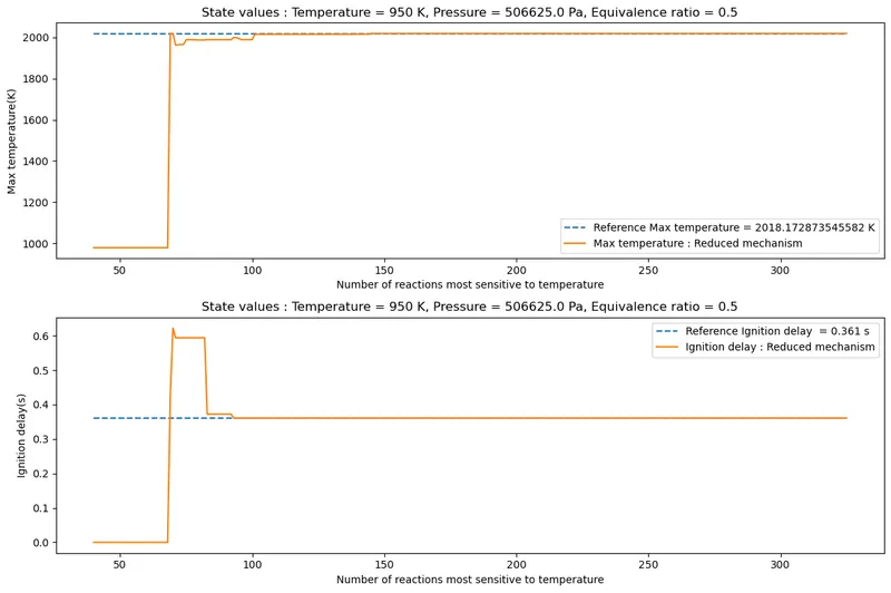
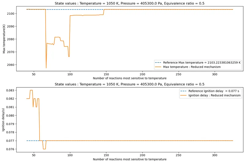
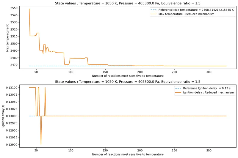
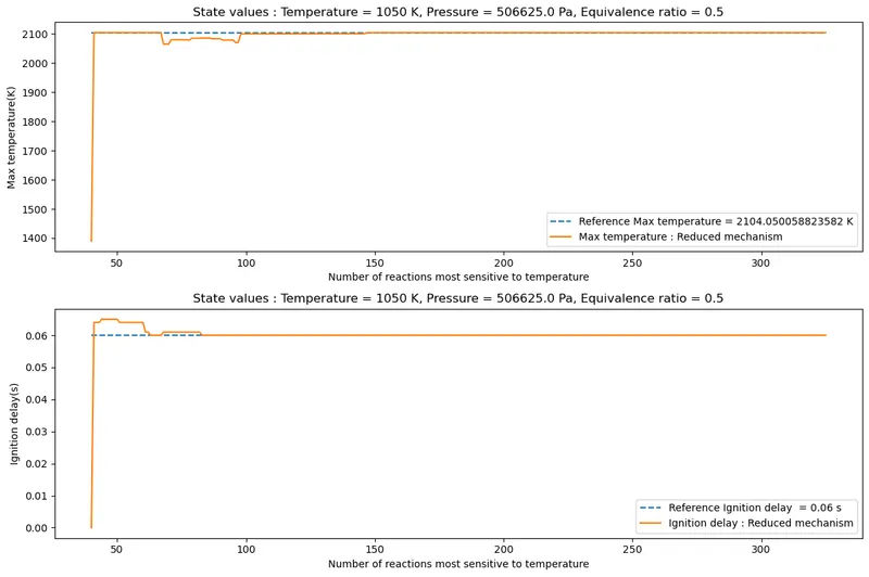
For fuel-rich mixtures, it can be seen that the maximum temperature after combustion does not vary significantly with the change in pressure(looking at each individual case). In the plots for the number of reactions vs maximum temperature for fuel-rich mixtures(`phi = 0.5`), it can be observed that the plots appear similar for each state value of temperature. Observing the fuel-rich plots of 950 K, it can be observed that the number of reactions required to obtain maximum temperature is the highest in the case with a pressure of 5 atm. This behaviour is observed at 950 K, and the other plots do not exhibit the same behaviour. The number of sensitive reactions needed before combustion begins increases as the equivalence ratio increases. At `P = 3 atm, phi = 0.5`, the number of reactions required for combustion to begin is around 50, while at `P = 5 atm, phi = 0.5`, the number of reactions required are around 70. The most reasonable explanation as to why this phenomenon occurs could be due to the possible relationship between pressure and the reaction rate of different reactions. It is known that the elementary reactions are dependent on other elementary reactions, and this influences the reaction rate of a reaction. Obtaining the most sensitive reaction is vital, but if the required reactants/radicals have not been produced from a relatively less sensitive reaction(the product of a less sensitive reaction), the presence of this reaction becomes meaningless.
This suggests that the rate of a highly sensitive reaction is directly influenced by the presence of an elementary reaction of relatively lower sensitivity, and the presence of this reaction is vital while creating a reduced mechanism file.
Increasing the base value of pressure influences the number of reactions and their respective reaction rates. This means that the pool of sensitive reactions increases with an increase in base temperature, becoming more dependent on each other, and hence, increasing the number of reactions required. This behaviour, however, is only observed at a temperature of 950 K. At 1050K and 1150K, this behaviour is not observed. But, the point made in this section will provide an insight as to what is happening in the other cases.
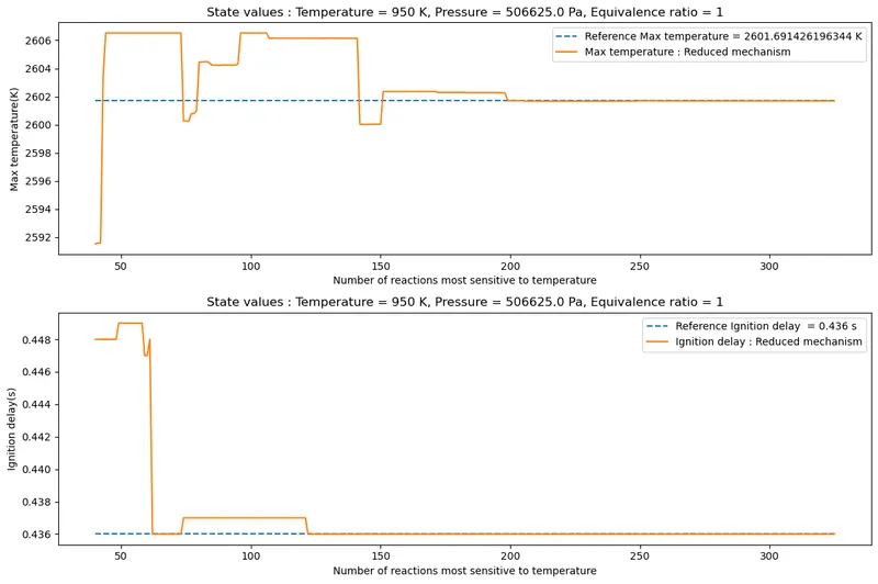
Another peculiar phenomenon that can be observed in the plots for the number of reactions vs maximum temperature is related to the initial pressure. At 4 atm pressure, it can be observed that the number of reactions required to obtain the maximum temperature is greater than both, 3 atm and 5 atm. This is true for all of the initial values of temperature. This suggests that a specific set of elementary reactions get involved at this temperature, and the effect of these reactions decreases as the initial pressure increases to 5 atm. It is reasonable to assume that there are a couple of reactions that negatively impact temperature increase, and these reactions dominate to a small extent at a pressure of 4 atm. The effect of these reactions, as mentioned above, decrease as the initial pressure is increased.
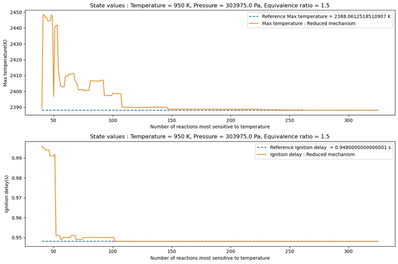
It should be noted that the number of reactions required to accurately capture the maximum temperature that can be achieved after the combustion of the mixture increases with the increase in temperature. This behaviour was expected, as the increase in initial temperature will increase the kinetic energy of the reactant species, which results in an increase in the rate of a reaction. The effect of the sensitive reactions becomes more apparent as the initial temperature increases. The reaction rates of previously dormant sensitive reactions increase to a great extent, increasing the number of chain-propagating reactions and chain-branching reactions. The chain-branching elementary reactions begin to play a bigger role as the initial temperature increases.
As mentioned previously, the maximum temperature does not vary to a great degree in the cases with `phi = 0.5`. The difference between each maximum temperature is around 1 Kelvin(varying initial pressure, keeping the initial temperature constant). The ignition delay, however, is affected greatly. The ignition delay decreases drastically with change in pressure. The decrease in ignition delay is most apparent at 950 K. At 1150 K, the effect is still present, but to a lesser extent. The increase in initial temperature does decrease the ignition delay, and combustion at 1150 K is easily the quickest. Despite the change being so great, the plots for the number of reactions vs ignition delay do not offer much in terms of determining the exact number of reactions required for obtaining a reaction mechanism capable of simulating combustion. Looking at the plots above, it can be said that around 50 to 100 sensitive reactions are required to accurately calculate the ignition delay. However, it should be noted that this range is not enough to capture the maximum temperature that can be achieved by the system, and hence, the plots of the number of sensitive reactions vs maximum temperature should be considered treated with more importance. The table below displays the number of reactions required to simulate combustion for each initial temperature value.
| Rich mixtures | Max temperature | Ignition Delay |
| `text(Temperature)` | `text(Number of reactions required)` | `text(Number of reactions required)` |
| `text(950 K)` | `120` | `100` |
| `text(1050 K)` | `150` | `90` |
| `text(1150 K)` | `170` | `80` |
For rich mixtures, around 170 reactions are required to obtain an accurate value of max temperature, and around 100 reactions are required to obtain an accurate value of ignition delay. However, 170 reactions are required to accurately simulate combustion. This will be explained in the final section.
It should be noted that this is the maximum number of reactions that should be considered, as the cases with lower initial temperatures require a lower number of reactions to simulate combustion.
Stoichiometric and lean mixtures:
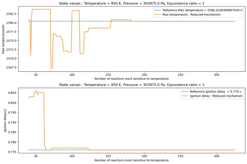
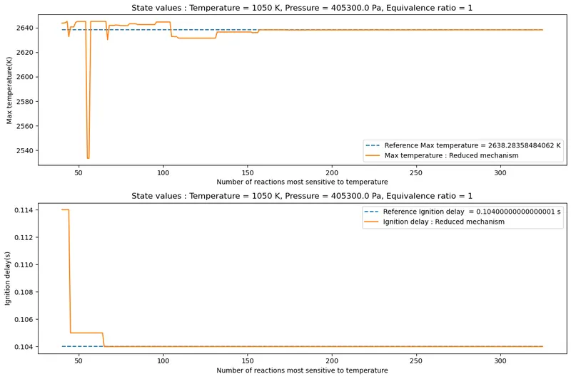
At 950 K, the plots for the number of reactions vs maximum temperature look strikingly similar, despite having different initial pressure values. The difference between each maximum temperature is around 10 Kelvin on average(varying initial pressure, keeping the initial temperature constant). The only temperature value for which this is not true is 1050 K. This seems to be an intermediate stage at which the trend that the plots for the number of reactions vs maximum temperature begin to change. At 950 K, it can be seen that the number of reactions required to simulate combustion increases with the increase in initial temperature. But for 1050 K and 1150 K, the opposite of this is true. The number of reactions required to simulate combustion reduces as the initial pressure is increased. This most likely occurs due to the increase in radical formation, as a stoichiometric mixture and a lean mixture will promote chain-propagating elementary reactions.
| Lean mixtures | Max temperature | Ignition Delay |
| `text(Temperature)` | `text(Number of reactions required)` | `text(Number of reactions required)` |
| `text(950 K)` | `240` | `110` |
| `text(1050 K)` | `210` | `100` |
| `text(1150 K)` | `200` | `100` |
| Stoichiometric mixtures | Max temperature | Ignition Delay |
| `text(Temperature)` | `text(Number of reactions required)` | `text(Number of reactions required)` |
| `text(950 K)` | `200` | `130` |
| `text(1050 K)` | `230` | `120` |
| `text(1150 K)` | `180` | `80` |
For lean mixtures, around 240 reactions are required to obtain an accurate value of max temperature, and around 110 reactions are required to obtain an accurate value of ignition delay. Using 240 reactions will accurately simulate combustion. Similarly, for stoichiometric mixtures, around 230 reactions are required to obtain an accurate value of max temperature, and around 130 reactions are required to obtain an accurate value of ignition delay. Using 230 reactions will accurately simulate combustion.
Discussion on the selection of the total number of reactions to be used in a reduced mechanism:
If the plots are observed, it can be seen that there are many plots in which the reference maximum temperature and ignition delay are achieved within the first 50 to 100 reactions. If a stopping criterion was implemented on this basis, this behaviour would not have been observed. There are reactions with negative sensitivity coefficients and these reactions would not have been taken into consideration. Hence, using taking into consideration the reactions after which there is no change whatsoever is important.
The ignition delay requires a low number of reactions in order to achieve an accurate value. If the objective is to obtain ignition delay without taking into consideration the maximum temperature, the minimum number of reactions required to obtain an accurate value of ignition delay for these state values is around 130.
The maximum temperature requires a significantly higher number of reactions to reach the reference max temperature value, and the minimum number of reactions required for this range of state values is around 240.
The highest number of the minimum number of reactions(considering the entire range of state values) has been selected for the reduced mechanism. This has been done to retain the accuracy for all ranges of state values. In summary, a minimum of 240 reactions will be required to accurately simulate combustion for this range of state values.