Conjugate Heat Transfer Analysis on a graphics card.

Aim : To perform a steady-state simulation on a graphics card, and observe the thermal effects of air velocity over the graphics card geometry.

Introduction:

Conjugate Heat Transfer analysis is used to capture accurate heat transfer behaviour due to both convection and conduction, for cases in which a solid and fluid at different temperatures or subjected to different thermal conditions interact with each other. This is especially useful at the fluid-solid interface, where the fluid interacts thermally with solid. The result obtained is a coupled solution, taking into account the thermal effects due to both, conduction and convection. It is also known for its flexibility, and its ability to handle complex simulations. Conjugate Heat Transfer can be used in a wide range of cases that involve mass-flow of a fluid over or inside a solid, subjected to different thermal conditions. Examples of the usage of CHT is seen in the determination of the effectiveness of heat transfer of a solid fin with a fluid flowing around it, fluid flowing through a tube at different temperature, such as a heat exchanger, and many more applications.

Theory:

A graphics card is primarily used to render images seen on the screen, and are known for performing more advanced tasks like running games and rendering 3D objects. The graphics card contains a processor, which performs tasks of this nature. Since performing all of these activities are computationally expensive, a lot of heat is generated by the processor. A graphics processor can generate heat up to 60 Watts, and the temperature of the processor increases to dangerously high levels. This high temperature may damage the components around it, and for this reason, the heat generated by it needs to be removed from the area. This can be done by cooling the processor using a fan or even liquid cooling. The effect of the velocity of the air used to cool the processor will be observed in this project.

Simulation workflow:

Setup details:

1. Inlet velocities considered: 1 m/s ,3 m/s and 5 m/s
2. Processor heat generation: 5 Watts

1.Geometry creation:

• The geometry of the graphics card was created using SpaceClaim.
• After the base geometry of the processor was created, the fluid domain within which air is meant to flow was created using the 'Enclosure' command. In order to obtain more accurate results, two enclosures were created. This will be elaborated upon further in the section detailing mesh creation.
• An issue that can be encountered during simulation due to the lack of cohesive geometry between the fluid domain and the solid domain, as the meshing suite will assume that these parts are separate. Due to this, the data obtained at the fluid and solid boundaries has a high chance of being unreliable.
• In order to avoid this issue, the 'Share Topology' option is enabled.

2. Mesh details:

Modelling approach:

• The objective of this simulation is to obtain the maximum temperature attained by the processor, the heat transfer coefficient of the processor and identify hotspots on the processor geometry.
• In order to carry out these objectives, the processor must be a source of heat generation. Hence, volumetric heat generation will be used on the processor body. A GPU processor can generate around 5 Watts of heat during normal operation, and this will be used as the value for heat generation. The volume of the processor will be taken into account, and this will be elaborated upon in the Fluent section.
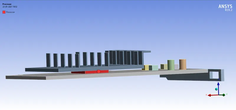
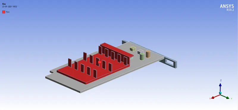
• Since the processor is the main source of heat, the components and the air in it's vicinity are bound to experience a temperature change. It should also be noted that the solids on the graphics card are different. The fins are made of aluminium, the card base is epoxy fiber-glass, and the processor is made of silicon. The heat transfer between different solids of different thermal characteristics require a higher degree of accuracy, and taking this fact into consideration, it is important that the mesh around the processor be of a higher mesh quality, in order to calculate the heat transfer between the different solid boundaries.
• The mesh quality of the fluid domain does not have to be extremely high, and some liberties can be taken with the mesh quality.

Mesh configuration:

The following methods were used to create the mesh for the graphics card geometry imported from Spaceclaim.

(I) Body sizing :

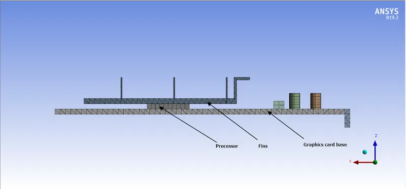
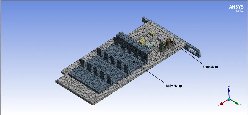
• The body sizing command is used by highlighting the processor, the fins and the card base and inserting the Body Sizing command. The element size was taken as 0.8 mm for the processor, and 1 mm for the fins and the card base. As stated above, this has been done in order to simulate accurate heat transfer by conduction at the boundaries of the different solid components.

(II) Edge sizing :

• The edge sizing command was used on the bodies resembling the capacitors on the card. The circumference of the cylindrical capacitors were selected, and edge sizing was inserted. The number of divisions on the selected edges were taken as 20. This has been done in order to smoothen the curvature of the cylindrical shape of the capacitor, and will ensure the prevention of any incorrectly simulated eddies in the vicinity during the simulation.

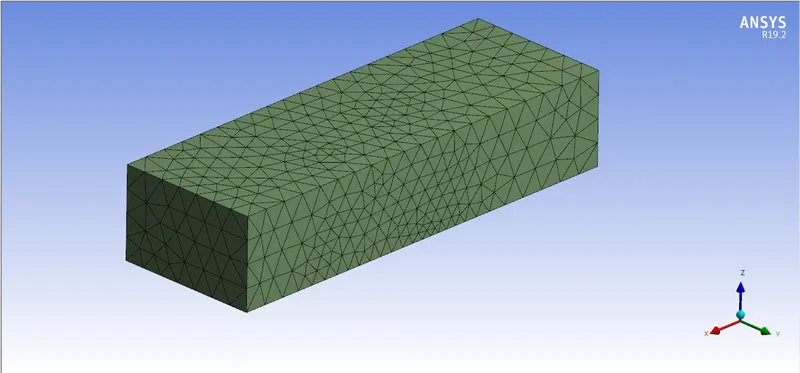
The fluid domain has been given an element size of 10 mm.

The following images show the mesh geometry:

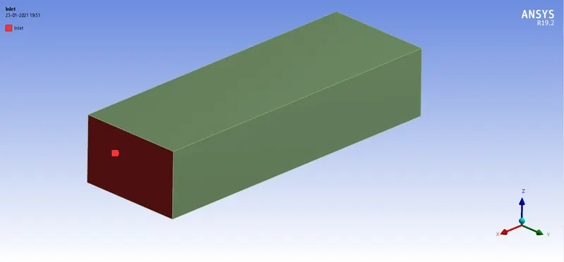
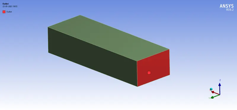
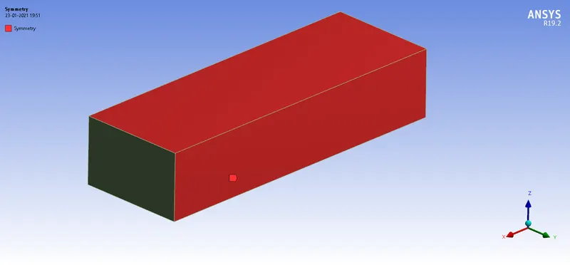
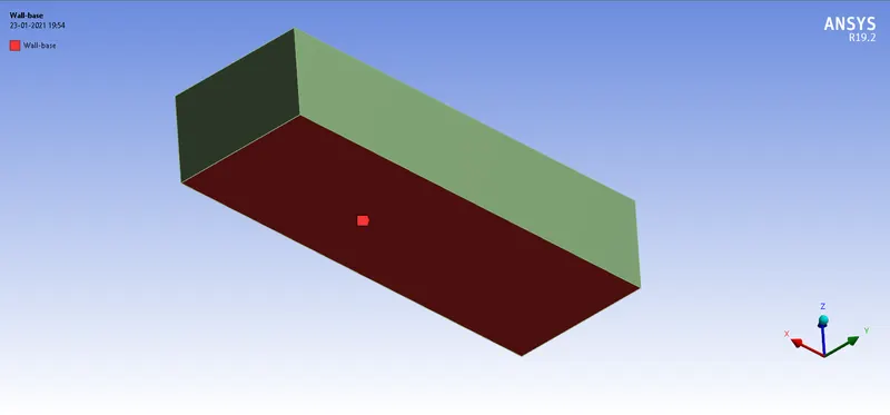
The named selections were provided by highlighting the required face and providing a suitable name. The inlet and outlet faces were specified, and the top,right and left faces of the fluid domain were specified as 'symmetry', as Fluent will automatically consider the symmetry boundary condition for these faces. The bottom face was set as a 'wall', and Fluent will automatically consider the base to be a wall.

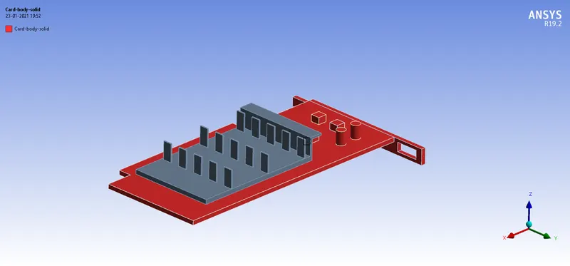
The processor, fins and card base geometries were given their respective names as well. This has been shown below.

3. Fluent setup

Solver setting: Pressure-based solver

A pressure-based solver is used for this case, and the compressibility effects are negligible in the flow. A density-based solver is highly accurate, but requires more computation time, and in this case, will not provide any significant advantage over a pressure based solver.

The energy equation is switched on.

Model used: k-omega SST

• The flow of the air over the graphics card is not laminar in nature, as flow separation will take place at many various locations of the card geometry.
• The k-omega SST model has been designed to combine the advantages of the k-epsilon and k-omega turbulence models. The k-omega model solves the near-wall functions accurately, but is inaccurate in the freestream velocity sections of the fluid flow, whereas the k-epsilon model accurately solves the freestream section of the fluid flow, but provides inaccurate values at the near wall or viscous sub-layer section.
• The k-omega SST model uses a k-epsilon model in the freestream sections of the fluid flow, and a k-omega model for near-wall computations. The ability of the k-omega SST model to resolve near-wall behaviour is imperative to attaining precise thermal behaviour near the inner wall.
• This seamless switching between models is done by the integration of two blending functions 'F1' and 'F2' in the equations of specific dissipation rate and kinematic eddy viscosity respectively.
• If the value of F1 is zero, the model switches to the k-epsilon model. Similarly, if the value of F1 is one, the k-omega model is used.
• F2 involves the use of a viscosity limiter, which prevents the model from over-predicting the wall shear stress, and functions similar to F1.

Pre-processing in Fluent:

General setup and turbulence model:

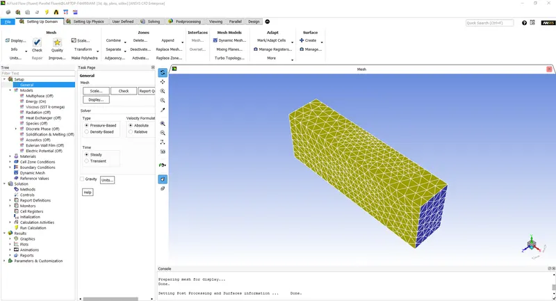
• The solver type and the steady state simulation options are set by going to Setup>General.
• The energy equation is turned on, as it is required in order to simulate heat transfer. This is done by going to Setup> Models > Energy Equation.
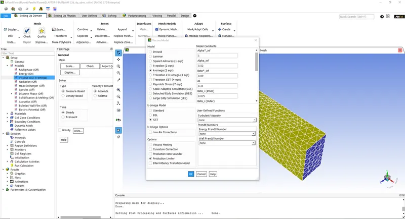
• The turbulence model is switched to k-omega SST by going to Setup> Models > Viscous, for the reasons stated above.
• The default fluid in fluent for the fluid is air, so no changes will be made to the material.

Materials:

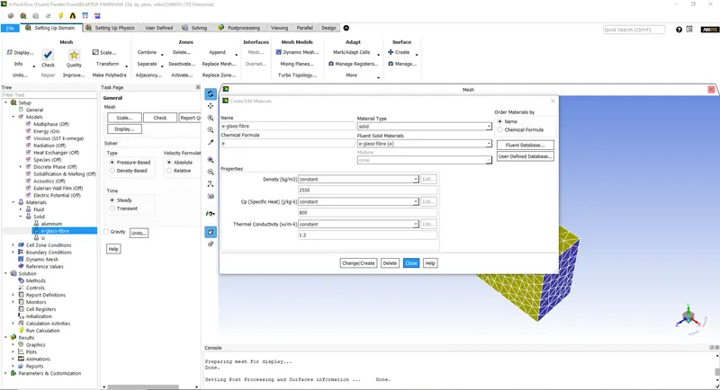
• Two new materials have been defined by going into Setup>Materials>Solid. The epoxy glass-fiber and the silcon materials are defined by providing their respective densities, thermal conductivities and their specific heat values.
• These materials are then created, and will be used for the card base and the processor respectively.

Cell zone conditions:

• The fluid and solid domains have been defined in this section.
• The processor, card base and the fins have been assigned silicon, epoxy glass-fiber and aluminium as their materials by entering Setup>Cell Zone Conditions.
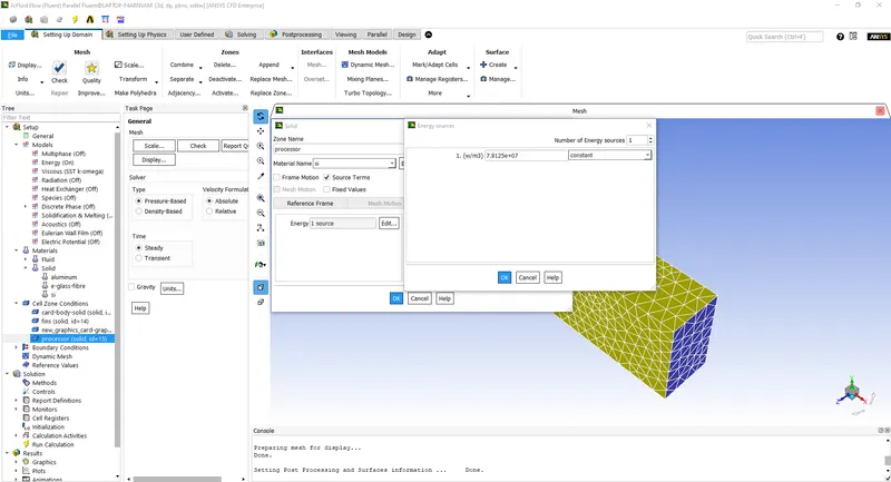
• An important point to note is that the processor has been considered as a volumetric heat generation source, and hence, the 'Source Term' option has been selected. The number of energy sources is set to one, and the volumetric heat generation in `W/m^3`, is then set. The amount of heat generated is taken as 5 Watts, and is divided by the volume of the processor, in order to obtain the volumetric heat generation. The computed value of heat generation is 7.8125e+07 `W/m^3`.

Boundary conditions:

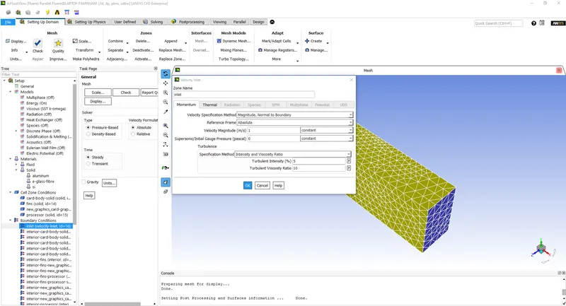
• Three cases will be run in this simulation. The freestream velocity of the air will be set as 1,3 and 5 m/s for their respective cases.
• The freestream velocity is set to 1,3 and 5 m/s at the inlet by going into Setup > Boundary Conditions > Inlet. The temperature of the fluid is changed in the same window by going to the Thermal settings in the same window, and is set to 298.15 Kelvin.
• The thermal boundary conditions of the inner wall is set to coupled.
• The boundary conditions of the simulation are under the same section under 'Type', and can be changed by using the dropdown provided below in the section.
• The boundary conditions are set in Fluent, as shown in the table below.

• Inlet	Velocity-inlet
  Outlet	Pressure-outlet
  Side walls	Symmetry
  Bottom	wall
  Processor	wall
  Card base	wall
  Fins	wall

• The number of iterations is set to 500 by entering the value within the Run calculation section.

Report and plot generation:

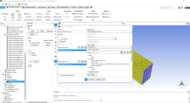
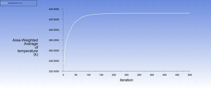
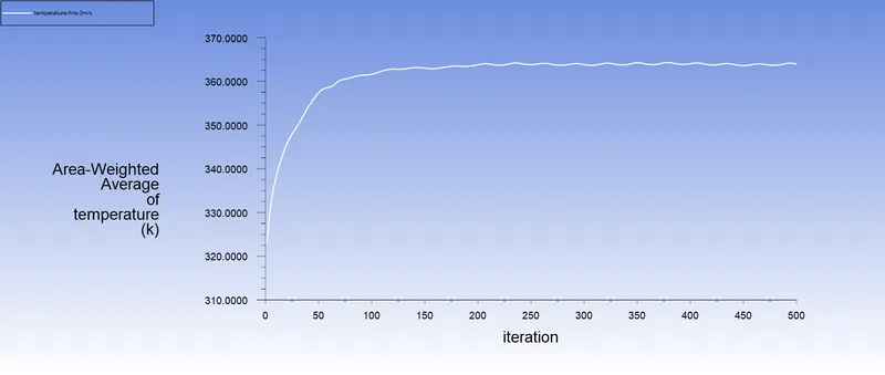
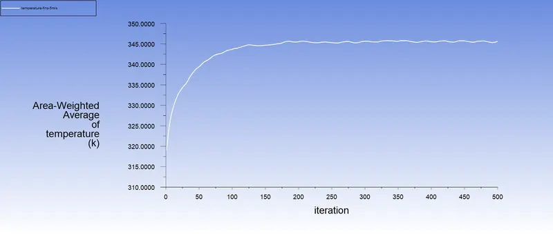
• A plot for the area-weighted average of the fins was created by entering Solution>Report Definitions. This will generate a plot of the same, and can be used as a reference to determine whether the solution has converged.

Post-processing:

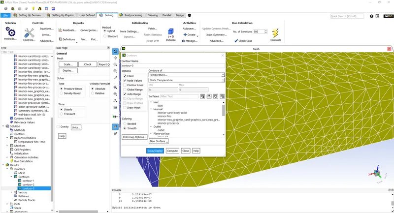
• The temperature contours can be obtained by entering Results > Graphics > Temperature>Static temperature, selecting the desired surface(in this case, the processor, fins and card base), and plotting the contour.
• The Surface Heat Transfer coefficient contours can be obtained by entering Results > Graphics > Wall Fluxes>Surface Heat Transfer Coefficient, selecting the desired surface(in this case, the processor, fins and card base), and plotting the contour.

The table below displays the steps mentioned above.

Results:

Temperature contours for a plane along the axis of the geometry:

Case	Temperature contours
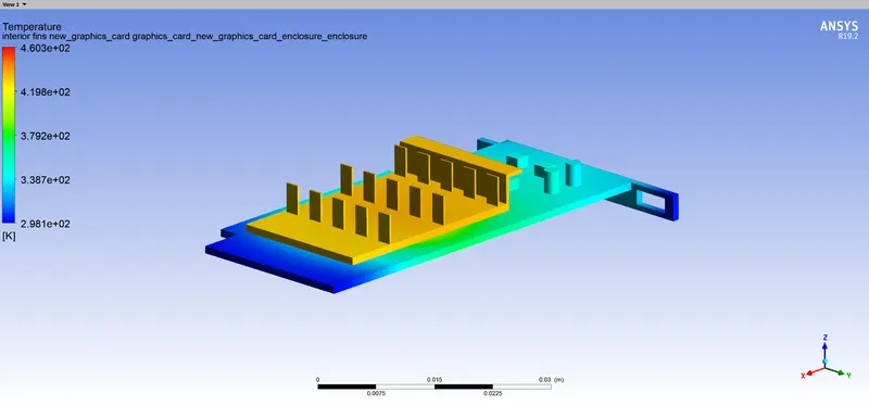
Case I: (Velocity=1m/s)
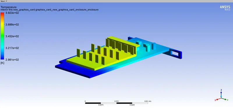
Case II: (Velocity=3m/s)
Case III: (Velocity=5m/s)

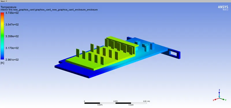Observing the temperature contours above, a couple of conclusions can be made.

As expected, the fins absorb a high quantity of heat generated by the processor and provides a larger surface area over which the heat has spread by conduction. Since aluminium is a good conductor of heat, the heat generated by the processor will flow into the aluminium fins. Some of the heat present in the fins is reduced due to convection, as the air flows over the fin geometry. This factor has a great effect on the amount of heat present in the graphics card.

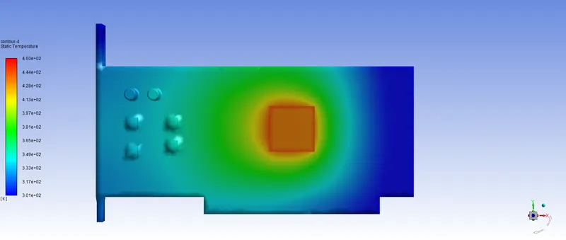
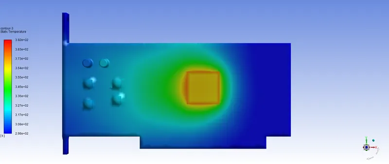
The temperature of the fins and the body itself, is higher the case with air velocity set at 1 m/s, compared to the cases with the air velocity set at 3 m/s and 5 m/s respectively. However, the volumetric heat generation of the processor is the same for all of the cases. So, it can be safely said that convection due to air flow over the body, plays a vital role in heat reduction in the graphics card. The maximum temperature achieved by the processor around 446 Kelvin when the freestream velocity of air is 1 m/s. This value of temperature is significantly higher compared to the temperatures achieved in the cases with the freestream air velocity set as 3 m/s and 5 m/s, 378 K and 360 K respectively.

It should also be noted that the temperature of the inlet air is set at 298.15 K for all of the cases.

The velocity of the air plays a vital role in understanding why the temperature of the fins reduces substantially. If the air around the fin were to remain still, or if the velocity of the air around the air was slow, the air would naturally heat up, and at a point, the heat transfer would reduce and equilibrium would be reached. However, if the air moves at a higher velocity, the air around the vicinity of the fins will always be at a lower temperature, as a fresh volume of air will replace the air present near the fins previously. The rate at which fresh room temperature air will replace the air in the vicinity of the fins is determined by the velocity of the air. Hence, heat present in the fins will be exhanged by convection at a faster rate, as the temperature difference between the air and the body will be larger in the cases with higher air velocity.

The following plots display the area-weighted average temperature of the processor, and shows that the solution has converged.

Case	Area-weighted average of temperature for aluminum fin
Case I : (Velocity=1m/s)
Case II: (Velocity=3m/s)
Case III: (Velocity=5m/s)

Heat Transfer Coefficient and temperature contour plots :

Case	Heat Transfer Coefficient contours
Case I : (Velocity=1m/s)
Case II: (Velocity=3m/s)
Case III: (Velocity=5m/s)

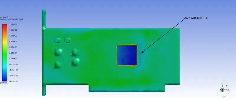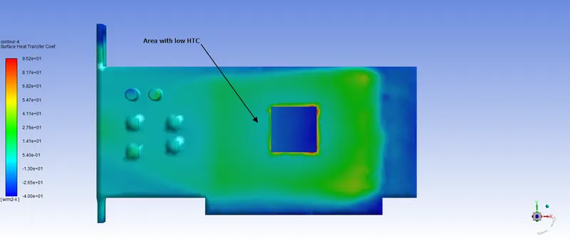
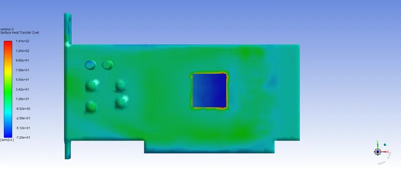
Observing the heat transfer coefficient plots above, two potential hotspots can be identified. The contours above display the HTC of the card base only, and the other parts have been disregarded for this section.

The first location that will be discussed is the area just beyond the processor, after the fluid flows over the processor. Upon observing the HTC contour of the case with a freestream velocity of 1 m/s, it can be seen that a low heat transfer coefficient is present in that area. A low heat transfer coefficient suggests that heat transfer is not taking place at a desirable rate in this area. This is area is important, as the heat generated by the processor should be taken away by the air, and cool down. But, this is not the case, as the closed nature of the geometry, and the low velocity contribute the heat remaining in that area. Flow separation takes place after the fluid crosses the processor, creating a low pressure region in that area. The low pressure region influences the fluid flowing around it, and the fluid in and around that volume slows down. Since the velocity of the air is extremely low in this region for the first case, the heat transfer by convection reduces and the region begins heating up. This phenomenon can be seen to great effect in the contour plot for temperature. The high temperature present in this area can cause damage to the components present in it's proximity.

However, this effect reduces with an increase in the freestream velocity of air. The average high speed of the air is enough to offset the effects of the flow separated zone for two reasons. Since the speed of the air is high, the low pressure zone that has been created behind the processor is unable to exert enough force on the fluid flowing just at the boundary of the flow separated zone. Due to this, the flow separated region does not grow larger in size, and hence, the effect of the flow separated region reduces.

The second hotspot that is identified can be seen in the cases with higher velocity. The high velocity air upon impinging the surface of the processor, decrease in velocity. This creates a high pressure zone, due to the impact. The fluid present in this zone exert a force on the fluid surround this area, and the velocity of the fluid around the zone increases. A positive pressure gradient is created at the edges of the processor, and the fluid velocity increases. However, the impact of the fluid on the processor causes the velocity to decrease in this area, and the fluid is unable to immediately rejoin the fluid flowing around it, as it does not possess the required energy. Since the velocity of the fluid has reduced, the heat transfer in this region reduces as well, creating a hotspot. The temperature contour plots displayed below show both of these hotspots.

Case	Temperature contours
Case I : (Velocity=1m/s)
Case II: (Velocity=3m/s)
Case III: (Velocity=5m/s)

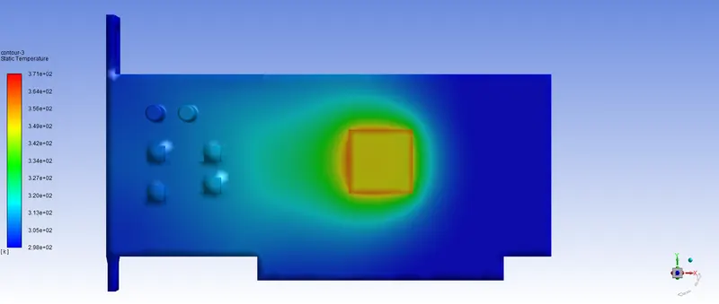From the plot shown above, it can be clearly seen that the temperature of the first hotspot zone reduces with increase in velcity.

The following vector plot displays the behaviour of the fluid with air velocity of 5 m/s.

Max temperature and heat transfer coefficient of the processor:

The maximum temperature attained by the processor was taken as the area-weighted average of the temperature of the processor, for all three cases. The following temperatures were obtained after computation. The maximum heat transfer coefficient has been displayed below as well and the following formula was used to obtain it.

`q = h*A*(T_(wall) - T_(ref))`

where,

`q = text(heat generated)`

`text(h = heat transfer coefficient)`

`text(A = Surface area of wall)`

`T_(wall) = text(temperature of the wall)`

`T_(ref) = text(temperature of the fluid at the inlet)`

Case	Max temperature(K)	Heat Transfer Coefficient`(W/m^2)`
Case I : (Velocity=1m/s)	446.287 K	21.095 `W/m^2`
Case II: (Velocity=3m/s)	378.970 K	38.666 `W/m^2`
Case III: (Velocity=5m/s)	360.627 K	50.017 `W/m^2`

Observing the values above, it can be concluded that the heat transfer coefficient increases with increase in freestream velocity. The heat generated by the processor is taken away by the air flowing over it, and increasing the velocity will result in an increase in the heat transfer by convection. This ultimately results in a lower processor temperature.

Conclusions:

Observing the results obtained after simulating three different cases with different values of inlet velocity, it can be concluded that the velocity of air over the geometry has a profound impact on the temperature of the processor, and the body itself. A higher value of air velocity will help maintain the health of the graphics card processor to a great degree, while a lower value of air velocity cannot prevent the processor from damaging the components around its proximity. Two main hotspots were observed after running the simulation, due to flow separation near the processor for the first case, and due to a high pressure zone caused by fluid(air) impingement on the processor body for the last two cases. The heat transfer coefficient and consequently, the heat transfer, will increase with an increase in freestream velocity.