The calculation of Adiabatic Flame Temperature in a Constant Volume Chamber using Python, and the effect of heat loss on the Adiabatic Flame Temperature of a gas.
AIM:
1. To observe the effect of equivalence ratio on the adiabatic flame temperature in a constant volume chamber by writing a program in python, and comparing the results obtained with cantera.
2. To calculate heat loss and observe its effect on adiabatic flame temperature of a gas.
Introduction:
The fuel-air equivalence ratio(`phi`) is the ratio of fuel to air corresponding to the actual conditions before combustion, to the fuel to air ratio corresponding to the stoichiometric condition of combustion of the fuel. The stoichiometric fuel to air ratio is the ratio of the exact amount of air required to combust all of the fuel provided. A standard fuel-to-oxidizer ratio is specific to the fuel used in the mixture, and hence, does not provide values that display the condition of the mixture for any type of fuel, except for the fuel considered. Observing the values of equivalence ratio,we can ascertain the type of mixture, regardless of the fuel that is considered. If the value of equivalence ratio is above 1, the mixture is rich, if it is below 1, the mixture is lean and if the value is equal to 1, the mixture is stoichiometric. The effect of the equivalence ratio of a mixture will be observed in this project.
Theory:
The Adiabatic Flame Temperature(AFT) of a fuel is the maximum temperature that can be achieved after complete combustion of all of the reactants in the system, with no heat transfer at the boundary. This means that the heat generated from combustion is utilized for the combustion products only, and there are no losses due to heat transfer at the boundaries. There are two types of Adiabatic Flame temperature:
(a) Constant Volume AFT
(b) Constant Pressure AFT
In the constant volume process, there is no heat transfer at the boundaries(Q=0) as the process is adiabatic and does not interact with the surroundings, and the work done in gas expansion post-combustion, is zero as well. This means that, if combustion took place inside a piston-cylinder arrangement, the piston would not move, as there is no work being done in order to move it. In this case, the difference between the internal energies of the products and the reactants, or vice versa, will be zero.
In the constant pressure process, the pressure is held constant, but unlike the constant volume process, work is done during gas expansion post-combustion, and the volume of the gas changes. A point to note is the fact that the constant volume adiabatic flame temperature should be higher than the constant temperature adiabatic flame temperature, because of the lack of work done in the constant volume process.
The adiabatic flame temperature of a fuel provides us with the maximum potential temperature that can be attained after the combustion of the fuel. This is important from a design perspective, as the materials chosen for the system in which combustion of this specific mixture takes place, should be able to withstand this temperature. Hence, designing the system considering the adiabatic flame temperature is beneficial.
The two expressions that will be used for CV-AFT and CP-AFT are as follows:
Constant Volume Adiabatic Flame Temperature:
H(reactants) - H(products) -R(n(reactants)*Tstd - n(products)*Tad) = 0
Constant Pressure Adiabatic Flame Temperature:
H(reactants) - H(products) = 0
where,
H(reactants) = Enthalpy of reactants(J)
H(products) = Enthalpy of products(J)
n(products) = number of moles of products
n(reactants) = number of moles of reactants(J)
Tstd = Initial Temperature(K) = 298.15 K
Tad = Adiabatic Temperature(K)
R = Gas constant = 8.313 J/K-mol
(I)Coding approach:
CASE I: To observe the effect of equivalence ratio on the adiabatic flame temperature in a constant volume chamber by writing a program in python, and comparing the results obtained with cantera.
For the constant volume adiabatic flame temperature calculation, the effect of the equivalence ratio on the AFT will be observed.
The following steps were performed in order to obtain the objective mentioned above:
Step 1:
Math,NumPy,Cantera and matplotlib were imported using the commands mentioned below.
Lines of code:
import math
import cantera as ct
import matplotlib.pyplot as plt
import numpy as np
The NASA polynomials have been used in order to obtain enthalpy.
Equation for enthalpy:
`H = (a1 + (a2*T/2) + (a3*(T^2)/3) + (a4*(T^3)/4) + (a5*(T^4)/5) + ((a6)/T))*R*T`
where,
H = Enthalpy(J)
T = Temperature(K)
(a1,a2,a3,a4,a5,a6) = Thermodynamic coefficients
The thermodynamic coefficients are given in the NASA thermodynamic files, where the first seven coefficients are for the high temperature range, and the last seven coefficients are for the lower temperature range. Inserting these values for a particular species will give us its enthalpy.
Example:
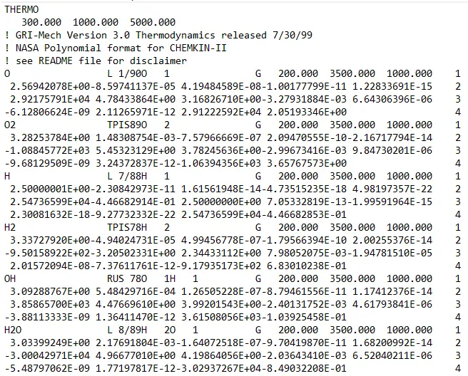
The coefficients are defined within the function 'h', and the function returns the enthalpy, taking temperature and the coefficient values as inputs.
Lines of code:
def h(T,coeff):
	R = 8.314
	a1 = coeff[0]
	a2 = coeff[1]
	a3 = coeff[2]
	a4 = coeff[3]
	a5 = coeff[4]
	a6 = coeff[5]

	return (a1 + (a2*T/2) + (a3*pow(T,2)/3) + (a4*pow(T,3)/4) + (a5*pow(T,4)/5) + (a6/T))*R*T
Step 2:
The coefficients for each species are defined and segregated into high temperature and low temperature coefficients. The low temperature coefficients are used for the reactants as they are at STP, pre-combustion. The high temperature coefficients are used for the products,as they are at a significantly higher temperature post-combustion. Since the combustion of methane is being observed, CH4,O2 and N2 are the reactants for which the low temperature coefficients will be used and H20,CO2,O2 and N2 will be the products. A point to note is that the combustion of stoichiometric and lean mixtures will be observed in this case, in order to obtain the trend of the equivalence ratio and the AFT. For this reason, O2 has been included in the products section only for lean mixtures, as the combustion of lean mixtures leaves some amount of air unreacted. This will be discussed in the next step.
The number of moles of fuel and air are specified for the actual condition and the stoichiometric condition, and consequently, the fuel-air ratios for both are obtained by inserting these values into their respective equations.
In order to obtain the behaviour of the adiabatic flame temperature with respect to the equivalence ratio, the number of moles of air will be a variable. An array for the number of moles of air is created by using the 'linspace' command in the NumPy library, and a range of required values are specified within it. The number of values required within said range is specified using 'num' within the bracket of the 'linspace' command.
The number of moles of air range from two to ten, two moles representing the stoichiometric condition, and the progressively becoming more lean in nature, as it approaches ten moles of air.
Lines of code:
#reactant coeffs
CH4_l_coeff = [5.14987613E+00,-1.36709788E-02, 4.91800599E-05,-4.84743026E-08, 1.66693956E-11,-1.02466476E+04,-4.64130376E+00]
O2_l_coeff = [3.78245636E+00,-2.99673416E-03, 9.84730201E-06,-9.68129509E-09, 3.24372837E-12,-1.06394356E+03, 3.65767573E+00]
N2_l_coeff = [0.03298677E+02, 0.14082404E-02,-0.03963222E-04,0.05641515E-07,-0.02444854E-10,-0.10208999E+04, 0.03950372E+02]
#product coeffs
CO2_h_coeff = [3.85746029E+00, 4.41437026E-03,-2.21481404E-06, 5.23490188E-10,-4.72084164E-14,-4.87591660E+04, 2.27163806E+00]
H20_h_coeff = [3.03399249E+00, 2.17691804E-03,-1.64072518E-07,-9.70419870E-11, 1.68200992E-14,-3.00042971E+04, 4.96677010E+00]
N2_h_coeff = [0.02926640E+02, 0.14879768E-02,-0.05684760E-05, 0.10097038E-09,-0.06753351E-13,-0.09227977E+04, 0.05980528E+02]
O2_h_coeff = [ 3.28253784E+00, 1.48308754E-03,-7.57966669E-07, 2.09470555E-10,-2.16717794E-14,-1.08845772E+03, 5.45323129E+00]


moles_of_fuel = 1
m_o_a = moles_of_air = np.linspace(2,10,num=15)
m_o_a_s = moles_of_air_stoichiometric = 2

far_stoi_cond = moles_of_fuel/moles_of_air_stoichiometric
far_actual_cond = moles_of_fuel/moles_of_air
Step 3:
The objective is to obtain the trend between the equivalence ratio and the AFT, so the formula for the equivalence ratio will be used as the main parameter. A 'for' loop is created in order to obtain multiple values of AFT, using the equivalance ratio as the 'range' of values for which the AFT is to be calculated. The formula contains the actual number of moles, which has been specified as a variable using 'linspace' as mentioned previously.
A function for the AFT at constant volume(equation mentioned above) is created within the 'for' loop, and uses temperature as an input.
The enthalpies for the different species are obtained by running the function for enthalpy mentioned above, and providing the temperature and thermodynamic coefficients of those specific species as inputs. The enthalpies of the reactants will use the temperature at STP and the low temperature coefficients, and the products will use the adiabatic flame temperature and the high temperature coefficients.
The total enthalpy for reactants and products are calculated by multiplying the number of moles that are present in the mixture for a specific species, before and after combustion respectively. The number of moles have been represented in terms of the equivalance ratio. The same has been done for the total number of moles.
For the number of moles of oxygen, we subtract the number of moles by 2, in order to consider the stoichiometric mixture. The combustion of a stoichiometric mixture does not yield excess oxygen as a product, and hence will be zero if this condition is satisfied. An important point to note is that this relation holds true only for stoichiometric and lean mixtures.
In order to store the values of AFT and equivalence ratio after every run of the 'for' loop, an empty array has been created outside the 'for' loop using the NumPy library, and will be called once again later.
Lines of code:
AFT_compilation =phi_compilation= np.array([])

for phi in (far_actual_cond/far_stoi_cond):
	def cv_func(T):
		#reactants
		R = 8.314
		Tstd = 298.15

		h_CH4_R = h(Tstd,CH4_l_coeff)
		h_O2_R = h(Tstd,O2_l_coeff)
		h_N2_R = h(Tstd,N2_l_coeff)
		h_CO2_P = h(T,CO2_h_coeff)
		h_H20_P = h(T,H20_h_coeff)
		h_N2_P = h(T,N2_h_coeff)
		h_O2_P = h(T,O2_h_coeff)

		#enthalpy and number of moles of reactants:
		H_reactants = h_CH4_R+ ((m_o_a_s/phi)*h_O2_R) + ((m_o_a_s/phi)*3.76*h_N2_R)
		n_reactants = 1 + (m_o_a_s/phi) + (m_o_a_s/phi)*3.76

		#enthalpy and number of moles of reactants:
		H_products = (h_CO2_P + 2*h_H20_P + ((m_o_a_s/phi)-2)*h_O2_P) + (m_o_a_s/phi*3.76*h_N2_P)
		n_products = 1 + 2 + ((m_o_a_s/phi)-2) + ((m_o_a_s/phi)*3.76)


		return (H_reactants - H_products) - (R*(n_reactants*Tstd - n_products*T))
Step 4:
The Newton-Raphson iterative method will be used in order to obtain the Adiabatic Flame Temperature.
Newton-Raphson method:
`x(n+1) = x(n) - (f(x)/(f'(x)))`
The denominator term is the numerical derivative of the function. Hence, using forward differencing, the numerical derivative of the function is obtained, and a function is created for the same, which uses temperature as an input.
The tolerance,initial guess for temperature,iteration number and the relaxation factor is set.
Lines of code:
	def f_numder(T):
		return (cv_func(T+1e-6) - cv_func(T))/(1e-6)

	tol = 1e-6
	T_guess = 1500
	iteration = 0
	alpha = 1
Step 5:
A 'while' loop is used in order to generate new guess values for adiabatic flame temperature, and is then inserted into the method mentioned above. The absolute value of the function is checked and compared with the tolerance value that has been set, and will stop only when the value of the function meets this criterion.
Hence, we get the adiabatic flame temperature after a few iterations.
The program runs until all of the values of AFT are obtained, for all of the values of the equivalence ratio, and then recall the array mentioned above to store all of the values generated in the loop, by using the 'append' command in NumPy. This is placed outside the 'while' loop, but within the 'for loop. This allows us to use the values for plotting purposes.
The values are then printed to the console.
Lines of code:
	while(abs((cv_func(T_guess)))>tol):
		T_guess = T_guess - alpha*(cv_func(T_guess))/f_numder(T_guess)

		iteration = iteration + 1

	AFT_compilation = np.append(AFT_compilation,T_guess)
	phi_compilation = np.append(phi_compilation,phi)

	print('Equivalence Ratio=','%.2f'%phi)
	print('Adiabatic Flame Temperature(constant volume)=',T_guess,'n')
print('n','n','n')
Step 6:[Cantera section]
In order to compare the values obtained by the program created above, the Cantera module is used obtain the AFT.
The 'ct.Solution('gri30.xml')' is used to obtain thermodynamic data. The gas is defined using this library, and is referred to as 'gas' in the program.
The same equation for equivalence ratio is used, as well the values of moles of fuel and air. The equivalance ratio is inserted in the 'for' loop as described above. The values of phi and AFT after every run of the 'for' loop will be stored in arrays as mentioned above, empty arrays outside the 'for' loop and recalled within the 'for' loop using the 'array' and 'append' commands respectively, utilizing the NumPy library.
The two commands that are specific to Cantera are 'TPX' and 'equilibrate'.
In Cantera, 'TPX' is used to set the temperature,pressure and mole fraction of the gas. The initial temperature is set at standard STP, and pressure at atmopheric pressure. The mole fraction of the species O2 and N2 utilize moles of air written in terms of phi, and the moles of fuel is set at 1 mole, as mentioned in the previous section.
The 'equilibrate' command is used for obtaining the temperature at equilibrium, ie.AFT. Within this command, 'UV' is selected in order to obtain the AFT at constant volume.
Hence, the values of AFT and phi are printed to the console.
Lines of code:
#program for adiabatic flame temperature using cantera:
gas = ct.Solution('gri30.xml')
#Arrays used to store the values of T_guess and equivalence ratio, after every pass of the 'for' loop.
AFT_compilation_cantera=phi_compilation_cantera=np.array([])

for phi in (far_actual_cond/far_stoi_cond):
	gas.TPX = 298.15,101325,{'CH4':moles_of_fuel,'O2':(m_o_a_s/phi), 'N2':(m_o_a_s/phi)*3.76}

	gas.equilibrate('UV',solver = 'auto')

	AFT_compilation_cantera = np.append(AFT_compilation_cantera,gas.T)
	phi_compilation_cantera = np.append(phi_compilation_cantera,phi)

	print('Equivalence Ratio[cantera]=','%.2f'%phi)
	print('Adiabatic Flame Temperature(constant volume)[cantera]=',gas.T,'n')
Step 7:
Plots for AFT vs equivalence ratio are created for both the program and cantera, using matplotlib.
The compiled values are used in order to create the plots.
The following matplotlib commands have been used to create the plot:
- plot : a line plot is created keeping the equivalence ratio on the X-axis, and the AFT on the Y-axis.
- scatter : a scatter plot is used to display the specific values which the program has computed, and is displayed with the line plot.
- grid: the grid is put on for displaying a grid on the plot.
- xlabel,ylabel : the axis is given a name in order to display the variable which it contains.
- title: a title is given to the plot.
- legend: a legend is created on the lower right side of the plot.
- show: the plot is displayed.
Lines of code:
#Comparison:
plt.plot(phi_compilation,AFT_compilation,label='AFT vs E.R: program',color = 'r')
plt.scatter(phi_compilation,AFT_compilation,color = 'r')
plt.plot(phi_compilation_cantera,AFT_compilation_cantera,label='AFT vs E.R: cantera',color = 'b')
plt.scatter(phi_compilation_cantera,AFT_compilation_cantera,color = 'b')
plt.grid('on')
plt.xlabel('Equivalence Ratio')
plt.ylabel('Adiabatic Flame Temperature(K)')
plt.title('AFT(K) vs Equivalence Ratio')
plt.legend(loc = 'lower right')
plt.show()
plt.show()
CASE II: To calculate heat loss and observe its effect on adiabatic flame temperature of a gas.
Step 1:
Math,NumPy,Cantera and matplotlib were imported using the commands mentioned below.
Lines of code:
import math
import cantera as ct
import matplotlib.pyplot as plt
import numpy as np
The NASA polynomials have been used in order to obtain enthalpy.
Equation for enthalpy:
`H = (a1 + (a2*T/2) + (a3*(T^2)/3) + (a4*(T^3)/4) + (a5*(T^4)/5) + ((a6)/T))*R*T`
where,
H = Enthalpy(J)
T = Temperature(K)
(a1,a2,a3,a4,a5,a6) = Thermodynamic coefficients
The thermodynamic coefficients are given in the NASA thermodynamic files, where the first seven coefficients are for the high temperature range, and the last seven coefficients are for the lower temperature range. Inserting these values for a particular species will give us its enthalpy.
The coefficients are defined within the function 'h', and the function returns the enthalpy, taking temperature and the coefficient values as inputs.
Lines of code:
def h(T,coeff):
	R = 8.314
	a1 = coeff[0]
	a2 = coeff[1]
	a3 = coeff[2]
	a4 = coeff[3]
	a5 = coeff[4]
	a6 = coeff[5]

	return (a1 + (a2*T/2) + (a3*pow(T,2)/3) + (a4*pow(T,3)/4) + (a5*pow(T,4)/5) + (a6/T))*R*T
Step 2:
Similar to step 2 of the previous section, the low and high temperature coefficients are defined for different species,with the exception being that the thermodynamic coefficients of ethane, ethene, ethyne and propane have been included in this case.
The overall heat transfer coefficient 'U' is specified, which represents the heat transfer at the boundaries. It is set at 500 for this case. The area is set at 1 m^2, the gas constant and the temperature at STP are set.
Lines of code:
#reactant coeffs
CH4_l_coeff = [5.14987613E+00,-1.36709788E-02, 4.91800599E-05,-4.84743026E-08, 1.66693956E-11,-1.02466476E+04,-4.64130376E+00]
C2H6_l_coeff = [4.29142492E+00,-5.50154270E-03, 5.99438288E-05,-7.08466285E-08, 2.68685771E-11,-1.15222055E+04, 2.66682316E+00]
C3H8_l_coeff = [0.93355381E+00, 0.26424579E-01, 0.61059727E-05,-0.21977499E-07, 0.95149253E-11,-0.13958520E+05, 0.19201691E+02]

C2H4_l_coeff = [3.95920148E+00,-7.57052247E-03, 5.70990292E-05,-6.91588753E-08, 2.69884373E-11, 5.08977593E+03, 4.09733096E+00]
C2H2_l_coeff = [8.08681094E-01, 2.33615629E-02,-3.55171815E-05,2.80152437E-08,-8.50072974E-12, 2.64289807E+04, 1.39397051E+01]
O2_l_coeff = [3.78245636E+00,-2.99673416E-03, 9.84730201E-06,-9.68129509E-09, 3.24372837E-12,-1.06394356E+03, 3.65767573E+00]
N2_l_coeff = [0.03298677E+02, 0.14082404E-02,-0.03963222E-04,0.05641515E-07,-0.02444854E-10,-0.10208999E+04, 0.03950372E+02]
#product coeffs
CO2_h_coeff = [3.85746029E+00, 4.41437026E-03,-2.21481404E-06, 5.23490188E-10,-4.72084164E-14,-4.87591660E+04, 2.27163806E+00]
H20_h_coeff = [3.03399249E+00, 2.17691804E-03,-1.64072518E-07,-9.70419870E-11, 1.68200992E-14,-3.00042971E+04, 4.96677010E+00]
N2_h_coeff = [0.02926640E+02, 0.14879768E-02,-0.05684760E-05, 0.10097038E-09,-0.06753351E-13,-0.09227977E+04, 0.05980528E+02]

U = 500
R = 8.314
Tstd = 298.15
A = 1
Step 3: Finding the AFT with heat loss of 0.35 of the total heat loss.
The heat loss is control using a coefficient named 'H_loss', and the value is set to 0.35.
A function for obtaining the AFT at constant pressure is created, and returns the solution to the equation mentioned in the theory section. The temperature and enthalpy are taken as inputs to this function. The enthalpies of the different species are obtained by using the function mentioned above, and hence, the total enthalpy of the reactants and products are obtained by adding the enthalpies of the different species. The enthalpies of the different species are multiplied by the number of moles they possess in the mixture.
The total heat loss is calculated by using the following relation:
Max heat loss = `U*A*(T-Tstd)`
where,
U = Overall Heat Transfer coefficient`(W/(m^2.K))` = 500
A = surface area(m^2)
T = adiabatic flame temperature
Tstd = 298.15 K
The Overall Heat Transfer Coefficient is set at 500.
The heat loss is controlled by multiplying the value of max heat loss with the coefficient mentioned above,this term is subtracted with the difference of the enthalpies of the reactants and the products, and the function returns the AFT with heat loss.
Lines of code:
#Case I: AFT of methane with heat loss of 0.35.

H_loss = 0.35
print('CASE I:')
def func_ch4(T):

	h_CH4_R = h(Tstd,CH4_l_coeff)
	h_O2_R = h(Tstd,O2_l_coeff)
	h_N2_R = h(Tstd,N2_l_coeff)
	#enthalpy reactants:
	H_reactants_CH4 = h_CH4_R+ (2*h_O2_R) + (7.52*h_N2_R)

	h_CO2_P = h(T,CO2_h_coeff)
	h_H20_P = h(T,H20_h_coeff)
	h_N2_P = h(T,N2_h_coeff)
	#enthalpy products:
	H_products_CH4 = (h_CO2_P + 2*h_H20_P + 7.52*h_N2_P)

	max_heat_loss = U*A*(T - Tstd)

	return (H_reactants_CH4 - H_products_CH4) - H_loss*(max_heat_loss)
The procedure to find the AFT is identical to the case mentioned previously.
The denominator term is the numerical derivative of the function. Hence, using forward differencing, the numerical derivative of the function is obtained, and a function is created for the same, which uses temperature as an input.
Lines of code:
def nd_ch4(T):
	return (func_ch4(T+1e-6) - func_ch4(T))/(1e-6)
The tolerance,initial guess for temperature,iteration number and the relaxation factor is set.
A 'while' loop is used in order to generate new guess values for adiabatic flame temperature, and is then inserted into the Newton- Raphson equation. The absolute value of the function is checked and compared with the tolerance value that has been set, and will stop only when the value of the function meets this criterion.
The values are then printed to the console.
Lines of code:
T_guess_ch4 = 1500
tol = 1e-6
alpha = 1
iteration = 0
while(abs(func_ch4(T_guess_ch4))>tol):
	T_guess_ch4 = T_guess_ch4 - alpha*(func_ch4(T_guess_ch4))/nd_ch4(T_guess_ch4)
	iteration = iteration + 1

print('AFT of Methane with heat loss of 0.35(of total heat loss) = ', T_guess_ch4,'K','n','n')
Step 4: Plotting a trend for heat loss and adiabatic flame temperature for Ethane,Ethene and Ethyne.
In order to achieve this objective, the heat loss will be used as a variable. A 'for' loop using heat loss coefficient values ranging from 0 to 1 has been created, and the AFT for different values of heat loss will be determined. The 'linspace' command in the NumPy library has been used for this purpose, and eleven values of heat loss coefficients between the given range have been specified within the 'linspace' command.
In order to store the values of AFTs of heat loss,Ethane, Ethene and Ethyne after every run of the 'for' loop, an empty array has been created outside the 'for' loop using the NumPy library.
The functions used to find the AFTs of Ethane, Ethene and Ethyne are defined, and the functions for the numerical derivatives of these functions are defined, identical to the procedure mentioned in the previous step. The initial guess values,tolerance, iteration number and the relaxation factor is set.
Lines of code:
#Case II: Plotting a trend for heat loss and adiabatic flame temperature for Ethane,Ethene and Ethyne:
#arrays used to compile AFTs and heat loss values:
t_ane=t_ene=t_yne=h_loss_comp=np.array([])
print('CASE II:')
for H_loss in np.linspace(0,1,num=11):
	h_loss_comp = np.append(h_loss_comp,H_loss)
	def func_c2h6(T):

		h_C2H6_R = h(Tstd,C2H6_l_coeff)
		h_O2_R = h(Tstd,O2_l_coeff)
		h_N2_R = h(Tstd,N2_l_coeff)

		h_CO2_P = h(T,CO2_h_coeff)
		h_H20_P = h(T,H20_h_coeff)
		h_N2_P = h(T,N2_h_coeff)

		#enthalpy reactants:
		H_reactants_C2H6 = h_C2H6_R+ (3.5*h_O2_R) + (13.16*h_N2_R)

		#enthalpy products:
		H_products_C2H6= (2*h_CO2_P + 3*h_H20_P + 13.16*h_N2_P)

		max_heat_loss = U*A*(T - Tstd)

		return (H_reactants_C2H6 - H_products_C2H6) - H_loss*(max_heat_loss)

	def func_c2h4(T):

		h_C2H4_R = h(Tstd,C2H4_l_coeff)
		h_O2_R = h(Tstd,O2_l_coeff)
		h_N2_R = h(Tstd,N2_l_coeff)

		h_CO2_P = h(T,CO2_h_coeff)
		h_H20_P = h(T,H20_h_coeff)
		h_N2_P = h(T,N2_h_coeff)

		#enthalpy reactants:
		H_reactants_C2H4 = h_C2H4_R + (3*h_O2_R) + (11.28*h_N2_R)

		#enthalpy products:
		H_products_C2H4= (2*h_CO2_P + 2*h_H20_P + 11.28*h_N2_P)

		max_heat_loss = U*A*(T - Tstd)

		return (H_reactants_C2H4 - H_products_C2H4) - H_loss*(max_heat_loss)


	def func_c2h2(T):

		h_C2H2_R = h(Tstd,C2H2_l_coeff)
		h_O2_R = h(Tstd,O2_l_coeff)
		h_N2_R = h(Tstd,N2_l_coeff)

		h_CO2_P = h(T,CO2_h_coeff)
		h_H20_P = h(T,H20_h_coeff)
		h_N2_P = h(T,N2_h_coeff)


		#enthalpy reactants:
		H_reactants_C2H2 = h_C2H2_R + (2.5*h_O2_R) + (9.3*h_N2_R)

		#enthalpy products:
		H_products_C2H2= (2*h_CO2_P + 1*h_H20_P + 9.3*h_N2_P)

		max_heat_loss = U*A*(T - Tstd)

		return (H_reactants_C2H2 - H_products_C2H2) - H_loss*(max_heat_loss)


	#Numerical derivative of temperature:
	def nd_c2h6(T):
		return (func_c2h6(T+1e-6) - func_c2h6(T))/(1e-6)

	def nd_c2h4(T):
		return (func_c2h4(T+1e-6) - func_c2h4(T))/(1e-6)

	def nd_c2h2(T):
		return (func_c2h2(T+1e-6) - func_c2h2(T))/(1e-6)


	#Initial guess:
	T_guess_c2h6 = T_guess_c2h4 = T_guess_c2h2 = 1500
	tol = 1e-6
	iteration = 0
	alpha = 1
A 'while' loop is used in order to generate new guess values for adiabatic flame temperature, and is then inserted into the Newton- Raphson equation. The absolute value of the function is checked and compared with the tolerance value that has been set, and will stop only when the value of the function meets this criterion. Separate 'while' loops have been created for Ethane,Ethene,and Ethyne and the values of AFT for different heat loss values are stored by using the 'append' command in the NumPy library, by recalling the empty arrays mentioned previously and inserting the values of AFT within these arrays.
The arrays that collect the AFTs for each species are placed after, but outside their respective 'while' loops.
The results are then printed to the console.
Lines of code:
	while(abs(func_c2h6(T_guess_c2h6))>tol):
		T_guess_c2h6 = T_guess_c2h6 - alpha*(func_c2h6(T_guess_c2h6))/nd_c2h6(T_guess_c2h6)
		iteration = iteration + 1

	t_ane = np.append(t_ane,T_guess_c2h6)

	while(abs(func_c2h4(T_guess_c2h4))>tol):
		T_guess_c2h4 = T_guess_c2h4 - alpha*(func_c2h4(T_guess_c2h4))/nd_c2h4(T_guess_c2h4)
		iteration = iteration + 1
	t_ene = np.append(t_ene,T_guess_c2h4)

	while(abs(func_c2h2(T_guess_c2h2))>tol):
		T_guess_c2h2 = T_guess_c2h2 - alpha*(func_c2h2(T_guess_c2h2))/nd_c2h2(T_guess_c2h2)
		iteration = iteration + 1
	t_yne = np.append(t_yne,T_guess_c2h2)


	print('Heat loss =','%.1f'%H_loss)
	print('%0s %21s %20s' %('AFT for ethane(K):','AFT for ethene(K):','AFT for ethyne(K):'))
	print('%0s %20s %20s' %(T_guess_c2h6,T_guess_c2h4,T_guess_c2h2),'n')
Step 5: COMPARISON BETWEEN CARBON ATOMS(1 to 3)
The procedure to find the AFT for Methane, Ethane, and Propane is identical to step 3. The only major difference in this case is that the heat loss in the system is zero. Hence, the plotting commands will be observed.
Lines of code:
while(abs(func_ch4(T_guess_ch4))>tol):
	T_guess_ch4 = T_guess_ch4 - alpha*(func_ch4(T_guess_ch4))/nd_ch4(T_guess_ch4)
	iteration = iteration + 1

while(abs(func_c2h6(T_guess_c2h6))>tol):
	T_guess_c2h6 = T_guess_c2h6 - alpha*(func_c2h6(T_guess_c2h6))/nd_c2h6(T_guess_c2h6)
	iteration = iteration + 1

while(abs(func_c3h8(T_guess_c3h8))>tol):
	T_guess_c3h8 = T_guess_c3h8 - alpha*(func_c3h8(T_guess_c3h8))/nd_c3h8(T_guess_c3h8)
	iteration = iteration + 1

print('%0s %20s %20s' %('AFT for methane:','AFT for ethane:','AFT for propane:'))
print('%0s %20s %20s' %(T_guess_ch4,T_guess_c2h6,T_guess_c3h8),'n')
Step 6: Plotting
Plotting commands used:
- figure: used to separate multiple figures if present.
- plot: it has been used to create a line plot for heat loss vs AFT, for Ethane,Ethene and Ethyne, and is figure(1).
- scatter: it has been used to create a scatter plot for number of carbon atoms vs AFT, for Methane,Ethane and Propane, and is figure(2).
- grid: the grid is put on for displaying a grid on the plot.
- xlabel,ylabel : the axis is given a name in order to display the variable which it contains.
- title: a title is given to the plot.
- legend: a legend is created on the lower right side of the plot for figure(2), and the default location is kept for figure(1)
- show: the plot is displayed.
Lines of code:
plt.figure(1)
plt.xlabel('Heat loss')
plt.ylabel('Adiabatic Flame Temperature(K)')
plt.title('Heat loss vs Adiabatic Flame Temperature(K)')
plt.plot(h_loss_comp,t_ane,label='Ethane',color ='r')
plt.plot(h_loss_comp,t_ene,label='Ethene',color='b')
plt.plot(h_loss_comp,t_yne,label='Ethyne',color='g')
plt.legend()
plt.grid()

plt.figure(2)
plt.xlabel('Number of carbon atoms')
plt.ylabel('Adiabatic Flame Temperature(K)')
plt.title('Number of carbon atoms vs AFT')
plt.scatter('Methane=1',T_guess_ch4,label='Methane',color='r')
plt.scatter('Ethane=2',T_guess_c2h6,label='Ethane',color='b')
plt.scatter('Propane=3',T_guess_c3h8,label='Propane',color='g')
plt.legend(loc='lower right')
#plt.plot(comp,temp,color='b')
plt.grid()
plt.show()
plt.show()
(II) Code:
The code for the first case has been shown below:
import math
import cantera as ct
import matplotlib.pyplot as plt
import numpy as np


def h(T,coeff):
	R = 8.314
	a1 = coeff[0]
	a2 = coeff[1]
	a3 = coeff[2]
	a4 = coeff[3]
	a5 = coeff[4]
	a6 = coeff[5]

	return (a1 + (a2*T/2) + (a3*pow(T,2)/3) + (a4*pow(T,3)/4) + (a5*pow(T,4)/5) + (a6/T))*R*T


#reactant coeffs
CH4_l_coeff = [5.14987613E+00,-1.36709788E-02, 4.91800599E-05,-4.84743026E-08, 1.66693956E-11,-1.02466476E+04,-4.64130376E+00]
O2_l_coeff = [3.78245636E+00,-2.99673416E-03, 9.84730201E-06,-9.68129509E-09, 3.24372837E-12,-1.06394356E+03, 3.65767573E+00]
N2_l_coeff = [0.03298677E+02, 0.14082404E-02,-0.03963222E-04,0.05641515E-07,-0.02444854E-10,-0.10208999E+04, 0.03950372E+02]
#product coeffs
CO2_h_coeff = [3.85746029E+00, 4.41437026E-03,-2.21481404E-06, 5.23490188E-10,-4.72084164E-14,-4.87591660E+04, 2.27163806E+00]
H20_h_coeff = [3.03399249E+00, 2.17691804E-03,-1.64072518E-07,-9.70419870E-11, 1.68200992E-14,-3.00042971E+04, 4.96677010E+00]
N2_h_coeff = [0.02926640E+02, 0.14879768E-02,-0.05684760E-05, 0.10097038E-09,-0.06753351E-13,-0.09227977E+04, 0.05980528E+02]
O2_h_coeff = [ 3.28253784E+00, 1.48308754E-03,-7.57966669E-07, 2.09470555E-10,-2.16717794E-14,-1.08845772E+03, 5.45323129E+00]


moles_of_fuel = 1
m_o_a = moles_of_air = np.linspace(2,10,num=15)
m_o_a_s = moles_of_air_stoichiometric = 2

far_stoi_cond = moles_of_fuel/moles_of_air_stoichiometric
far_actual_cond = moles_of_fuel/moles_of_air

#equivalence ratio:
#phi = actual fuel-air ratio/stoichiometric fuel-air ratio = moles of air(stoichiometric)/moles of air

#Arrays used to store the values of T_guess and equivalence ratio, after every pass of the 'for' loop.
AFT_compilation =phi_compilation= np.array([])

for phi in (far_actual_cond/far_stoi_cond):
	def cv_func(T):
		#reactants
		R = 8.314
		Tstd = 298.15

		h_CH4_R = h(Tstd,CH4_l_coeff)
		h_O2_R = h(Tstd,O2_l_coeff)
		h_N2_R = h(Tstd,N2_l_coeff)
		h_CO2_P = h(T,CO2_h_coeff)
		h_H20_P = h(T,H20_h_coeff)
		h_N2_P = h(T,N2_h_coeff)
		h_O2_P = h(T,O2_h_coeff)

		#enthalpy and number of moles of reactants:
		H_reactants = h_CH4_R+ ((m_o_a_s/phi)*h_O2_R) + ((m_o_a_s/phi)*3.76*h_N2_R)
		n_reactants = 1 + (m_o_a_s/phi) + (m_o_a_s/phi)*3.76

		#enthalpy and number of moles of reactants:
		H_products = (h_CO2_P + 2*h_H20_P + ((m_o_a_s/phi)-2)*h_O2_P) + (m_o_a_s/phi*3.76*h_N2_P)
		n_products = 1 + 2 + ((m_o_a_s/phi)-2) + ((m_o_a_s/phi)*3.76)


		return (H_reactants - H_products) - (R*(n_reactants*Tstd - n_products*T))

	def f_numder(T):
		return (cv_func(T+1e-6) - cv_func(T))/(1e-6)

	tol = 1e-6
	T_guess = 1500
	iteration = 0
	alpha = 1


	while(abs((cv_func(T_guess)))>tol):
		T_guess = T_guess - alpha*(cv_func(T_guess))/f_numder(T_guess)

		iteration = iteration + 1

	AFT_compilation = np.append(AFT_compilation,T_guess)
	phi_compilation = np.append(phi_compilation,phi)

	print('Equivalence Ratio=','%.2f'%phi)
	print('Adiabatic Flame Temperature(constant volume)=',T_guess,'n')
print('n','n','n')


#program for adiabatic flame temperature using cantera:
gas = ct.Solution('gri30.xml')
#Arrays used to store the values of T_guess and equivalence ratio, after every pass of the 'for' loop.
AFT_compilation_cantera=phi_compilation_cantera=np.array([])

for phi in (far_actual_cond/far_stoi_cond):
	gas.TPX = 298.15,101325,{'CH4':moles_of_fuel,'O2':(m_o_a_s/phi), 'N2':(m_o_a_s/phi)*3.76}

	gas.equilibrate('UV',solver = 'auto')

	AFT_compilation_cantera = np.append(AFT_compilation_cantera,gas.T)
	phi_compilation_cantera = np.append(phi_compilation_cantera,phi)

	print('Equivalence Ratio[cantera]=','%.2f'%phi)
	print('Adiabatic Flame Temperature(constant volume)[cantera]=',gas.T,'n')

#Comparison:
plt.plot(phi_compilation,AFT_compilation,label='AFT vs E.R: program',color = 'r')
plt.scatter(phi_compilation,AFT_compilation,color = 'r')
plt.plot(phi_compilation_cantera,AFT_compilation_cantera,label='AFT vs E.R: cantera',color = 'b')
plt.scatter(phi_compilation_cantera,AFT_compilation_cantera,color = 'b')
plt.grid('on')
plt.xlabel('Equivalence Ratio')
plt.ylabel('Adiabatic Flame Temperature(K)')
plt.title('AFT(K) vs Equivalence Ratio')
plt.legend(loc = 'lower right')
plt.show()
plt.show()
The code for the second case has been shown below:
import math
import cantera as ct
import matplotlib.pyplot as plt
import numpy as np

def h(T,coeff):
	R = 8.314
	a1 = coeff[0]
	a2 = coeff[1]
	a3 = coeff[2]
	a4 = coeff[3]
	a5 = coeff[4]
	a6 = coeff[5]

	return (a1 + (a2*T/2) + (a3*pow(T,2)/3) + (a4*pow(T,3)/4) + (a5*pow(T,4)/5) + (a6/T))*R*T


#reactant coeffs
CH4_l_coeff = [5.14987613E+00,-1.36709788E-02, 4.91800599E-05,-4.84743026E-08, 1.66693956E-11,-1.02466476E+04,-4.64130376E+00]
C2H6_l_coeff = [4.29142492E+00,-5.50154270E-03, 5.99438288E-05,-7.08466285E-08, 2.68685771E-11,-1.15222055E+04, 2.66682316E+00]
C3H8_l_coeff = [0.93355381E+00, 0.26424579E-01, 0.61059727E-05,-0.21977499E-07, 0.95149253E-11,-0.13958520E+05, 0.19201691E+02]

C2H4_l_coeff = [3.95920148E+00,-7.57052247E-03, 5.70990292E-05,-6.91588753E-08, 2.69884373E-11, 5.08977593E+03, 4.09733096E+00]
C2H2_l_coeff = [8.08681094E-01, 2.33615629E-02,-3.55171815E-05,2.80152437E-08,-8.50072974E-12, 2.64289807E+04, 1.39397051E+01]
O2_l_coeff = [3.78245636E+00,-2.99673416E-03, 9.84730201E-06,-9.68129509E-09, 3.24372837E-12,-1.06394356E+03, 3.65767573E+00]
N2_l_coeff = [0.03298677E+02, 0.14082404E-02,-0.03963222E-04,0.05641515E-07,-0.02444854E-10,-0.10208999E+04, 0.03950372E+02]
#product coeffs
CO2_h_coeff = [3.85746029E+00, 4.41437026E-03,-2.21481404E-06, 5.23490188E-10,-4.72084164E-14,-4.87591660E+04, 2.27163806E+00]
H20_h_coeff = [3.03399249E+00, 2.17691804E-03,-1.64072518E-07,-9.70419870E-11, 1.68200992E-14,-3.00042971E+04, 4.96677010E+00]
N2_h_coeff = [0.02926640E+02, 0.14879768E-02,-0.05684760E-05, 0.10097038E-09,-0.06753351E-13,-0.09227977E+04, 0.05980528E+02]

U = 500
R = 8.314
Tstd = 298.15
A = 1

#Case I: AFT of methane with heat loss of 0.35.

H_loss = 0.35
print('CASE I:')
def func_ch4(T):

	h_CH4_R = h(Tstd,CH4_l_coeff)
	h_O2_R = h(Tstd,O2_l_coeff)
	h_N2_R = h(Tstd,N2_l_coeff)
	#enthalpy reactants:
	H_reactants_CH4 = h_CH4_R+ (2*h_O2_R) + (7.52*h_N2_R)

	h_CO2_P = h(T,CO2_h_coeff)
	h_H20_P = h(T,H20_h_coeff)
	h_N2_P = h(T,N2_h_coeff)
	#enthalpy products:
	H_products_CH4 = (h_CO2_P + 2*h_H20_P + 7.52*h_N2_P)

	max_heat_loss = U*A*(T - Tstd)

	return (H_reactants_CH4 - H_products_CH4) - H_loss*(max_heat_loss)

def nd_ch4(T):
	return (func_ch4(T+1e-6) - func_ch4(T))/(1e-6)

T_guess_ch4 = 1500
tol = 1e-6
alpha = 1
iteration = 0
while(abs(func_ch4(T_guess_ch4))>tol):
	T_guess_ch4 = T_guess_ch4 - alpha*(func_ch4(T_guess_ch4))/nd_ch4(T_guess_ch4)
	iteration = iteration + 1

print('AFT of Methane with heat loss of 0.35(of total heat loss) = ', T_guess_ch4,'K','n','n')

#Case II: Plotting a trend for heat loss and adiabatic flame temperature for Ethane,Ethene and Ethyne:

#arrays used to compile AFTs and heat loss values:
t_ane=t_ene=t_yne=h_loss_comp=np.array([])
print('CASE II:')
for H_loss in np.linspace(0,1,num=11):
	h_loss_comp = np.append(h_loss_comp,H_loss)
	def func_c2h6(T):

		h_C2H6_R = h(Tstd,C2H6_l_coeff)
		h_O2_R = h(Tstd,O2_l_coeff)
		h_N2_R = h(Tstd,N2_l_coeff)

		h_CO2_P = h(T,CO2_h_coeff)
		h_H20_P = h(T,H20_h_coeff)
		h_N2_P = h(T,N2_h_coeff)

		#enthalpy reactants:
		H_reactants_C2H6 = h_C2H6_R+ (3.5*h_O2_R) + (13.16*h_N2_R)

		#enthalpy products:
		H_products_C2H6= (2*h_CO2_P + 3*h_H20_P + 13.16*h_N2_P)

		max_heat_loss = U*A*(T - Tstd)

		return (H_reactants_C2H6 - H_products_C2H6) - H_loss*(max_heat_loss)

	def func_c2h4(T):

		h_C2H4_R = h(Tstd,C2H4_l_coeff)
		h_O2_R = h(Tstd,O2_l_coeff)
		h_N2_R = h(Tstd,N2_l_coeff)

		h_CO2_P = h(T,CO2_h_coeff)
		h_H20_P = h(T,H20_h_coeff)
		h_N2_P = h(T,N2_h_coeff)

		#enthalpy reactants:
		H_reactants_C2H4 = h_C2H4_R + (3*h_O2_R) + (11.28*h_N2_R)

		#enthalpy products:
		H_products_C2H4= (2*h_CO2_P + 2*h_H20_P + 11.28*h_N2_P)


		max_heat_loss = U*A*(T - Tstd)

		return (H_reactants_C2H4 - H_products_C2H4) - H_loss*(max_heat_loss)


	def func_c2h2(T):

		h_C2H2_R = h(Tstd,C2H2_l_coeff)
		h_O2_R = h(Tstd,O2_l_coeff)
		h_N2_R = h(Tstd,N2_l_coeff)

		h_CO2_P = h(T,CO2_h_coeff)
		h_H20_P = h(T,H20_h_coeff)
		h_N2_P = h(T,N2_h_coeff)


		#enthalpy reactants:
		H_reactants_C2H2 = h_C2H2_R + (2.5*h_O2_R) + (9.3*h_N2_R)

		#enthalpy products:
		H_products_C2H2= (2*h_CO2_P + 1*h_H20_P + 9.3*h_N2_P)

		max_heat_loss = U*A*(T - Tstd)

		return (H_reactants_C2H2 - H_products_C2H2) - H_loss*(max_heat_loss)


	#Numerical derivative of temperature:
	def nd_c2h6(T):
		return (func_c2h6(T+1e-6) - func_c2h6(T))/(1e-6)

	def nd_c2h4(T):
		return (func_c2h4(T+1e-6) - func_c2h4(T))/(1e-6)

	def nd_c2h2(T):
		return (func_c2h2(T+1e-6) - func_c2h2(T))/(1e-6)


	#Initial guess:
	T_guess_c2h6 = T_guess_c2h4 = T_guess_c2h2 = 1500

	tol = 1e-6
	iteration = 0
	alpha = 1


	while(abs(func_c2h6(T_guess_c2h6))>tol):
		T_guess_c2h6 = T_guess_c2h6 - alpha*(func_c2h6(T_guess_c2h6))/nd_c2h6(T_guess_c2h6)
		iteration = iteration + 1

	t_ane = np.append(t_ane,T_guess_c2h6)

	while(abs(func_c2h4(T_guess_c2h4))>tol):
		T_guess_c2h4 = T_guess_c2h4 - alpha*(func_c2h4(T_guess_c2h4))/nd_c2h4(T_guess_c2h4)
		iteration = iteration + 1
	t_ene = np.append(t_ene,T_guess_c2h4)

	while(abs(func_c2h2(T_guess_c2h2))>tol):
		T_guess_c2h2 = T_guess_c2h2 - alpha*(func_c2h2(T_guess_c2h2))/nd_c2h2(T_guess_c2h2)
		iteration = iteration + 1
	t_yne = np.append(t_yne,T_guess_c2h2)


	print('Heat loss =','%.1f'%H_loss)
	print('%0s %21s %20s' %('AFT for ethane(K):','AFT for ethene(K):','AFT for ethyne(K):'))
	print('%0s %20s %20s' %(T_guess_c2h6,T_guess_c2h4,T_guess_c2h2),'n')


#Case III :COMPARISON BETWEEN CARBON ATOMS(1 to 3):
H_loss = 0
print('CASE III:')
def func_ch4(T):

	h_CH4_R = h(Tstd,CH4_l_coeff)
	h_O2_R = h(Tstd,O2_l_coeff)
	h_N2_R = h(Tstd,N2_l_coeff)
	#enthalpy reactants:
	H_reactants_CH4 = h_CH4_R+ (2*h_O2_R) + (7.52*h_N2_R)

	h_CO2_P = h(T,CO2_h_coeff)
	h_H20_P = h(T,H20_h_coeff)
	h_N2_P = h(T,N2_h_coeff)
	#enthalpy products:
	H_products_CH4 = (h_CO2_P + 2*h_H20_P + 7.52*h_N2_P)

	max_heat_loss = U*A*(T - Tstd)

	return (H_reactants_CH4 - H_products_CH4) - H_loss*(max_heat_loss)

def func_c2h6(T):

	h_C2H6_R = h(Tstd,C2H6_l_coeff)
	h_O2_R = h(Tstd,O2_l_coeff)
	h_N2_R = h(Tstd,N2_l_coeff)

	h_CO2_P = h(T,CO2_h_coeff)
	h_H20_P = h(T,H20_h_coeff)
	h_N2_P = h(T,N2_h_coeff)

	#enthalpy reactants:
	H_reactants_C2H6 = h_C2H6_R+ (3.5*h_O2_R) + (13.16*h_N2_R)

	#enthalpy products:
	H_products_C2H6= (2*h_CO2_P + 3*h_H20_P + 13.16*h_N2_P)

	max_heat_loss = U*A*(T - Tstd)

	return (H_reactants_C2H6 - H_products_C2H6) - H_loss*(max_heat_loss)

def func_c3h8(T):

	h_C3H8_R = h(Tstd,C3H8_l_coeff)
	h_O2_R = h(Tstd,O2_l_coeff)
	h_N2_R = h(Tstd,N2_l_coeff)
	#enthalpy reactants:
	H_reactants_C3H8 = h_C3H8_R+ (5*h_O2_R) + (18.8*h_N2_R)

	h_CO2_P = h(T,CO2_h_coeff)
	h_H20_P = h(T,H20_h_coeff)
	h_N2_P = h(T,N2_h_coeff)
	#enthalpy products:
	H_products_C3H8 = (3*h_CO2_P + 4*h_H20_P + 18.8*h_N2_P)
	max_heat_loss = U*A*(T - Tstd)

	return (H_reactants_C3H8 - H_products_C3H8) - H_loss*(max_heat_loss)

def nd_ch4(T):
	return (func_ch4(T+1e-6) - func_ch4(T))/(1e-6)

def nd_c2h6(T):
	return (func_c2h6(T+1e-6) - func_c2h6(T))/(1e-6)

def nd_c3h8(T):
	return (func_c3h8(T+1e-6) - func_c3h8(T))/(1e-6)

T_guess_ch4 = T_guess_c3h8 = 1500
tol = 1e-6
iteration = 0
alpha = 1

while(abs(func_ch4(T_guess_ch4))>tol):
	T_guess_ch4 = T_guess_ch4 - alpha*(func_ch4(T_guess_ch4))/nd_ch4(T_guess_ch4)
	iteration = iteration + 1

while(abs(func_c2h6(T_guess_c2h6))>tol):
	T_guess_c2h6 = T_guess_c2h6 - alpha*(func_c2h6(T_guess_c2h6))/nd_c2h6(T_guess_c2h6)
	iteration = iteration + 1

while(abs(func_c3h8(T_guess_c3h8))>tol):
	T_guess_c3h8 = T_guess_c3h8 - alpha*(func_c3h8(T_guess_c3h8))/nd_c3h8(T_guess_c3h8)
	iteration = iteration + 1


print('%0s %20s %20s' %('AFT for methane:','AFT for ethane:','AFT for propane:'))
print('%0s %20s %20s' %(T_guess_ch4,T_guess_c2h6,T_guess_c3h8),'n')


plt.figure(1)
plt.xlabel('Heat loss')
plt.ylabel('Adiabatic Flame Temperature(K)')
plt.title('Heat loss vs Adiabatic Flame Temperature(K)')
plt.plot(h_loss_comp,t_ane,label='Ethane',color ='r')
plt.plot(h_loss_comp,t_ene,label='Ethene',color='b')
plt.plot(h_loss_comp,t_yne,label='Ethyne',color='g')
plt.legend()
plt.grid()

plt.figure(2)
plt.xlabel('Number of carbon atoms')
plt.ylabel('Adiabatic Flame Temperature(K)')
plt.title('Number of carbon atoms vs AFT')
plt.scatter('Methane=1',T_guess_ch4,label='Methane',color='r')
plt.scatter('Ethane=2',T_guess_c2h6,label='Ethane',color='b')
plt.scatter('Propane=3',T_guess_c3h8,label='Propane',color='g')
plt.legend(loc='lower right')
#plt.plot(comp,temp,color='b')
plt.grid()
plt.show()
plt.show()
(III) Results:
CASE I: To observe the effect of equivalence ratio on the adiabatic flame temperature in a constant volume chamber by writing a program in python, and comparing the results obtained with cantera.
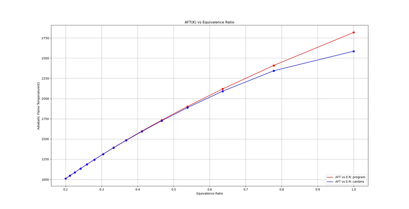
- In a constant volume chamber, the adiabatic flame temperature is high, since no work is being done. For stoichiometric to increasingly lean mixtures, the adiabatic flame temperature varies linearly with the equivalence ratio. The higher the equivalence ratio, the higher the adiabatic flame temperature. This trend is seen in both, the AFT obtained by creating a program that calculates it manually, and the cantera module.
- However, when the results of the program are compared with cantera, it can be observed that the program over-predicts the AFT by a fair amount. The AFT at phi = 1, is around 2817 K, whereas the AFT obtained using cantera is around 2585 K.
- But, as the value of phi decreases, the accuracy of the program increases, to a point where the values of AFT obtained by both, the program and Cantera, are identical.
- The reason behind this simple. The program over-predicts the AFT when the equivalance ratio is 1, because the species provided are simply not enough, as the products of combustion generated are far more than three products. The more products, the more energy would be distributed among them. Since the program contains only three products, the heat energy is distributed among these three, giving a higher value of AFT. The Cantera module is able to distribute the heat energy throughout all of the products of combustion,and this is the limitation of the program created, as we cannot manually gauge the number of moles of each minor product created post-combustion.
- The program gives more accurate values of AFT as the equivalence ratio decreases, as the amount of oxygen in the products post-combustion increases, the leaner a mixture becomes. The excess air becomes a main product of combustion, and at the near the lowest equivalence ratio, we can see that the values of AFT are identical for the program and Cantera. The minor products produced have very little effect on the AFT,as their production severely reduces as the mixture becomes leaner.
- The following plot displays this behaviour:
Console display: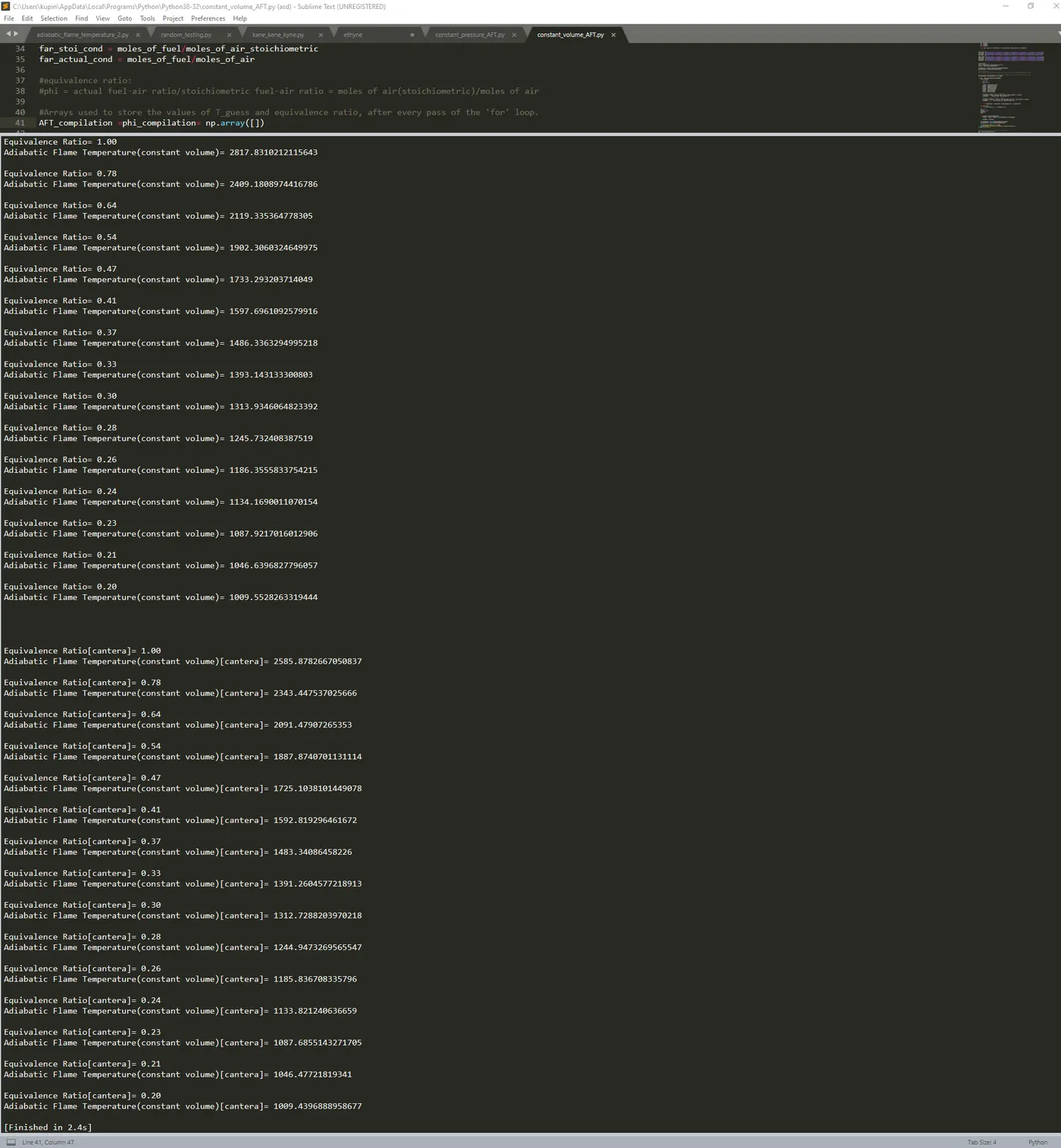
CASE II: To calculate heat loss and observe its effect on adiabatic flame temperature of a gas
(1) AFT of methane with heat loss coefficient of 0.35(35% of total heat loss):
- The AFT of methane as anticipated, decreases with the introduction of a heat loss value. The AFT of methane with heat loss is found to be 1744.05 K.
(2) Plotting a trend for heat loss and adiabatic flame temperature for Ethane,Ethene and Ethyne:
- The following plot displays Heat loss vs AFT.
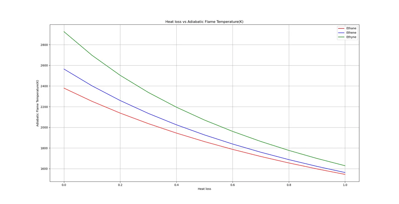
- From the plot above, it can be observed that the AFT is highly affected by heat loss, and the temperature reduces significantly as the heat loss values increase. However the most drastic drop is observed in Ethyne, as the values of heat loss increase for Ethyne, the AFT reduces far more aggressively compared to Ethane and Ethene.
- The increase in heat loss causes the AFTs of Ethane,Ethene and Ethyne to have values nearer to each other, compared to the values of AFT with no heat loss.
- Hence, heat loss and AFT are inversely proportional,as the increase of the heat loss coefficient causes a decrease in the AFT.
- A point to note is that the AFT of Ethyne is excessively over-predicted by the program. The combustion of Ethyne yields the most uncombusted air, and the increase in the number of moles of other minor products. Hence, the results should be observed only for their behaviour with heat loss.
(3) Increasing the number of carbon atoms, and observing its effect on the AFT:
The following scatter plot displays the increase of carbon atoms vs AFT.
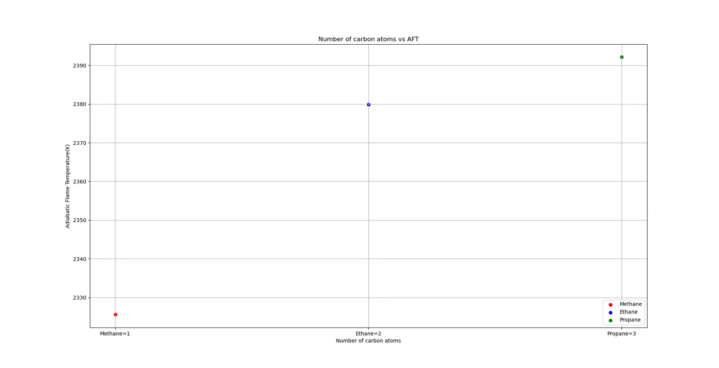
- From the above plot, it can be observed that the increase in carbon atoms results in an increase in the AFT.
- However, the increase in the adiabatic flame temperature is marginal. All three fuels lie within the 2300K to 2400K range, especially in the case of Ethane and Propane, where there is only a 13K difference between their AFTs.
Console display: 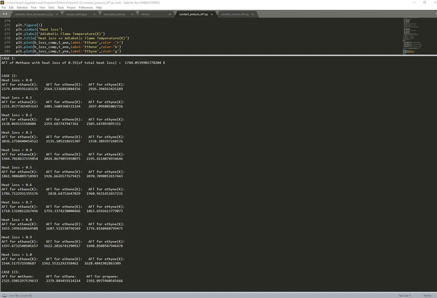
Google drive link for programs:
https://drive.google.com/drive/folders/1rqVRrXayiYhI40AeuyKONXX81EQtEmLh?usp=sharing