The application of the Newton-Raphson multivariate method and the Implicit Euler’s method on a system of coupled non-linear Ordinary Differential Equations.
Aim : To implement the Implicit Euler method(Backward differencing method), while employing the Newton-Raphson method to solve the system of coupled non-linear equations, and obtaining the ideal time step for the simulation.
Introduction:
Systems of ordinary differential equations are observed in physics and chemistry. For practical applications, solving complex ordinary differential equations relating to a specific field is time consuming. Most of the time, analytical solutions for these equations are too tedious and require a high amount of computational effort. Numerical methods mitigate this issue, as they provide faster approximate solutions and are relatively easier on computational effort. Different numerical methods offer different advantages and disadvantages in terms of accuracy, computational time and effort, and are applied considering the type of problem. Solving these equations as efficiently and accurately as possible is a necessity, and using the correct numerical method is paramount. Different numerical methods offer different levels of accuracy and computational speed. The Implicit Euler method is a first order numerical method, but offers a high level of stability. However, implementing this method becomes slightly more complex with a system of coupled ordinary differential equations. In order to overcome this obstacle, the Newton-Raphson method has been utilized. This method is an iterative technique that is capable of solving a system of coupled ordinary differential equations. The Implicit Euler method is an L-stable method, and can accomodate large time step sizes, while providing a solution that will not break down. This does not mean that the solution obtained is an accurate solution. Hence, the selection of the time step size is important, and the factors influencing the time step size will be discussed in this project.
Theory:
The implicit Euler method will be utilized to obtain the numerical solutions of the given system of ODEs. It is a first order numerical method,i.e. the error obtained is of the first order. As previously mentioned, this method is an L-stable method, and the solution will not break down, despite the implementation of a large time step size. This is the biggest advantage of this method. However, the accuracy of the numerical solution is compromised with the use of a large time step size. This method utilizes the values of the next time step in order to solve the functions in the ODEs. However, we do not have the values of the next time step required to compute the numerical solution. The Newton-Raphson method has been utilized to compute these values iteratively, using the values of the current time step, and guess values for the next time step. This will be elaborated upon in the coding section, as it will provide a clearer understanding of this situation.
The time step will be computed with respect to the tolerance required, and the relation between the error and the time step will be discussed in the results section.
Formulae:
Implicit Euler method:
`y_i = y_((i-1)) + dt*f(t_i,y_i)`
`dy/(dt) = y' = f(t,y)`
where,
`dt = text(time step size)`
`i = text(time step)`
Newton-Raphson method:
`y_(n+1) = y_n - (alpha*(J(y_n))^-1*F(y_n))`
where,
`J = text(Jacobian matrix)`
`F= text(Vector Function)`
`n = text(iteration)`
ODEs to be solved:
`dy_1/(dt) = -0.04*(y_1) + (10^4*y_2*y_3)`
`dy_2/(dt)= 0.04*y_1 - (10^4*y_2*y_3) - (3*10^7*y_2^2)`
`dy_3/(dt) = (3*10^7*y_2^2)`
ODEs after the implementation of the Implicit Euler method:
`y_1(i) =y_1(i-1) + dt*( -0.04*(y_1(i)) + (10^4*y_2(i)*y_3(i)))`
`y_2(i) = y_2(i-1) + dt*(0.04*y_1(i) - (10^4*y_2(i)*y_3(i)) - (3*10^7*(y_2(i))^2))`
`y_3(i) = y_3(i-1) + dt*(3*10^7*(y_2(i))^2)`
Simulation time:
10 minutes(600 seconds)
Initial values of `y_1,y_2` and `y_3`:
`y_1 = 1`
`y_2 = 0`
`y_3 = 0`
Coding Approach:
The coding approach for the program is as follows.
Step I: Importing libraries
- The NumPy, numpy.linalg and matplotlib libraries are imported into the program by using the 'import' command.
Lines of code:
import numpy as np
import matplotlib.pyplot as plt
from numpy.linalg import inv
Step II: Creating a function for the Vector Function
- In order to create the vector function, the ODEs have been re-arranged in a way that will resemble a root-finding problem. The equations have been listed below.
`f_1 =y_1(i-1) - y_1(i) + dt*( -0.04*(y_1(i)) + (10^4*y_2(i)*y_3(i))) = 0`
`f_2 = y_2(i-1) - y_2(i) + dt*(0.04*y_1(i) - (10^4*y_2(i)*y_3(i)) - (3*10^7*(y_2(i))^2))=0`
`f_3 = y_3(i-1) - y_3(i) + dt*(3*10^7*(y_2(i))^2) = 0`
- Three functions have been created for the functions mentioned above, and taking the values of `y_1,y_2` and `y_3` at the current time step, the values of `y_1,y_2` and `y_3` at the next time step and time step size as required arguments. If the lines of code are observed, the values of y1,y2 and y3 for the next time step have been written as y1_guess,y2_guess, and y3_guess. This will be elaborated upon in step 4.
- But, to explain superficially, this has been done in order to obtain the values of `y_1,y_2` and `y_3` for the next time step, using the Newton-Raphson multivariate method.
- The functions will return `f_1,f_2` and `f_3` respectively.
Lines of code:
#Functions for the Vector function
def f1(y1,y1_guess,y2_guess,y3_guess,dt):
	return  y1 - (y1_guess) + dt*(-0.04*(y1_guess) + pow(10,4)*(y2_guess)*(y3_guess))

def f2(y2,y1_guess,y2_guess,y3_guess,dt):
	return y2 - (y2_guess) + dt*(0.04*(y1_guess) - pow(10,4)*(y2_guess)*(y3_guess) - (3*pow(10,7)*pow(y2_guess,2)))

def f3(y3,y1_guess,y2_guess,y3_guess,dt):
	return y3 - (y3_guess) + dt*(3*pow(10,7)*pow(y2_guess,2))
Step III: Partial differentiation of `f_1,f_2,f_3` with respect to `y_1,y_2,y_3` using the central difference method.
- The Jacobian used in the Newton-Raphson method contains partial derivatives of `f_1,f_2,f_3` with respect to `y_1,y_2,y_3`. The central difference method has been utilized for the partially differentiating the functions, and is second-order accurate.
- This has been done by perturbing the variable that is being partially differenced, while keeping the remaining variables unchanged. The value with which the variable is being perturbed is kept sufficiently small, in order to ensure high accuracy.
- The following example will make the implementation of this method clearer.
`(delf_1)/(dely_1) = (f_1[t,y_1(i-1),(y_1(i)+h),y_2(i),y_3(i)] - f_1[t,y_1(i-1),(y_1(i)-h),y_2(i),y_3(i)])/(2*h)`
where,
`h = text(step size of perturbation)`
- Functions for all of the partial derivatives required for the Jacobian have been created, taking the values of `y_1,y_2` and `y_3` at the current time step, the values of `y_1,y_2` and `y_3` at the next time step,step size of perturbation(h) and time step size as required arguments.
- The functions will return the partial derivatives of the vector function with respect to `y_1,y_2` and `y_3`.
Lines of code:
#Partial differentiation using central differencing method:
#First Row:
def df1_dy1(y1,y1_guess,y2_guess,y3_guess,h,dt):
	return (f1(y1,(y1_guess+h),y2_guess,y3_guess,dt) - f1(y1,(y1_guess-h),y2_guess,y3_guess,dt))/(2*h)

def df1_dy2(y1,y1_guess,y2_guess,y3_guess,h,dt):
	return (f1(y1,y1_guess,(y2_guess+h),y3_guess,dt) - f1(y1,y1_guess,(y2_guess-h),y3_guess,dt))/(2*h)

def df1_dy3(y1,y1_guess,y2_guess,y3_guess,h,dt):
	return (f1(y1,y1_guess,y2_guess,(y3_guess+h),dt) - f1(y1,y1_guess,y2_guess,(y3_guess-h),dt))/(2*h)

#Second Row:
def df2_dy1(y2,y1_guess,y2_guess,y3_guess,h,dt):
	return (f2(y2,(y1_guess+h),y2_guess,y3_guess,dt) - f2(y2,(y1_guess-h),y2_guess,y3_guess,dt))/(2*h)

def df2_dy2(y2,y1_guess,y2_guess,y3_guess,h,dt):
	return (f2(y2,y1_guess,(y2_guess+h),y3_guess,dt) - f2(y2,y1_guess,(y2_guess-h),y3_guess,dt))/(2*h)

def df2_dy3(y2,y1_guess,y2_guess,y3_guess,h,dt):
	return (f2(y2,y1_guess,y2_guess,(y3_guess+h),dt) - f2(y2,y1_guess,y2_guess,(y3_guess-h),dt))/(2*h)

#Third Row
def df3_dy1(y3,y1_guess,y2_guess,y3_guess,h,dt):
	return (f3(y3,(y1_guess+h),y2_guess,y3_guess,dt) - f3(y3,(y1_guess-h),y2_guess,y3_guess,dt))/(2*h)

def df3_dy2(y3,y1_guess,y2_guess,y3_guess,h,dt):
	return (f3(y3,y1_guess,(y2_guess+h),y3_guess,dt) - f3(y3,y1_guess,(y2_guess-h),y3_guess,dt))/(2*h)

def df3_dy3(y3,y1_guess,y2_guess,y3_guess,h,dt):
	return (f3(y3,y1_guess,y2_guess,(y3_guess+h),dt) - f3(y3,y1_guess,y2_guess,(y3_guess-h),dt))/(2*h)
Step IV : The Jacobian
- A `3times 3` matrix has been created, as there are 9 possible partial derivatives that have to be computed. This has been done by using the 'ones' function of the NumPy library, and the number of columns and rows have been specified within this function.
- The function will return a `3times 3` matrix of ones.
- Since this is a list data type, each item can be replaced with a required value. In this case, the items of the matrix will be partial derivatives of the vector function, differentiated with respect to `y_1,y_2,y_3`. The Jacobian has been displayed below.
`J = [[(delf_1)/(dely_1),(delf_1)/(dely_2),(delf_1)/(dely_3)],[(delf_2)/(dely_1),(delf_2)/(dely_2),(delf_2)/(dely_3)],[(delf_3)/(dely_1),(delf_3)/(dely_2),(delf_3)/(dely_3)]]`
- The functions created for the partial derivatives(mentioned in step III), are inserted into their respective positions inside the matrix.
- The function created for this Jacobian will take the values of `y_1,y_2` and `y_3` at the current time step, the values of `y_1,y_2` and `y_3` at the next time step,step size of perturbation(h) and time step size as required arguments.
- The function will return the Jacobian matrix that has been created.
Lines of code:
#Jacobian:
def jacobian(y1,y2,y3,y1_guess,y2_guess,y3_guess,h,dt):
	J = np.ones((3,3))
	J[0,0] = df1_dy1(y1,y1_guess,y2_guess,y3_guess,h,dt)
	J[0,1] = df1_dy2(y1,y1_guess,y2_guess,y3_guess,h,dt)
	J[0,2] = df1_dy3(y1,y1_guess,y2_guess,y3_guess,h,dt)
	J[1,0] = df2_dy1(y2,y1_guess,y2_guess,y3_guess,h,dt)
	J[1,1] = df2_dy2(y2,y1_guess,y2_guess,y3_guess,h,dt)
	J[1,2] = df2_dy3(y2,y1_guess,y2_guess,y3_guess,h,dt)
	J[2,0] = df3_dy1(y3,y1_guess,y2_guess,y3_guess,h,dt)
	J[2,1] = df3_dy2(y3,y1_guess,y2_guess,y3_guess,h,dt)
	J[2,2] = df3_dy3(y3,y1_guess,y2_guess,y3_guess,h,dt)
	return J
Step V: Implementation of Implicit Euler's method and Newton-Raphson method
SET-UP EXPLANATION :
- This step contains the main part of this project. The concepts implemented will be elaborated upon here.
- The Implicit Euler method utilizes that values of the next time step to compute the function within it, in order to calculate the values at the next time step. Of course, these values are not known to us. Re-arranging the equations will yield no helpful result, as the equations cannot be decoupled manually. However, the initial values of `y_1,y_2` and `y_3` at the initial time step are known to us.
- It is for this precise reason that the Newton-Raphson multivariate method will be utilized. The Newton-Raphson multivariate method is an iterative technique used to find the roots of an equation. For clarity, the vector functions will be listed below.
`f_1 =y_1(i-1) - y_1(i) + dt*( -0.04*(y_1(i)) + (10^4*y_2(i)*y_3(i))) = 0`
`f_2 = y_2(i-1) - y_2(i) + dt*(0.04*y_1(i) - (10^4*y_2(i)*y_3(i)) - (3*10^7*(y_2(i))^2))=0`
`f_3 = y_3(i-1) - y_3(i) + dt*(3*10^7*(y_2(i))^2) = 0`
- Speaking in terms of the first time step, it can be observed that the initial values are known to us, as stated above. That leaves three unknowns in the three functions. If the values of the three unknowns(`y_1,y_2` and `y_3` at the next time step), are guessed, we can utilize the Newton-Raphson method.For reference, the formula for N-R multivariate method will be displayed below, in the way it will be utilized in the program.
`y_(text(new guess)) = y_(guess) - (alpha*(J(y_(guess)))^-1*F(y_(guess)))`
- The old guess values will utilize the user defined guess values initially. The Jacobian and the vector function will be computed using the guess values. Once a new guess value has been obtained using the Newton-Raphson method, it will be compared to the old guess value by running the values in a stopping criterion, which contains the tolerance criterion. If the difference between the values does not meet the required tolerance, the new guess value will be utilized as a guess value. Since this is an iterative process, it will continue until the stopping criterion is satisfied. Once the stopping criterion has been fulfilled, the process will stop, and the correct values of `y_1,y_2` and `y_3` at the next time step will be obtained, for a specific time step.
- To put it simply, the final guess values that satisfy the stopping criterion, are the correct values of `y_1,y_2` and `y_3` for the next time step.
- Since a solution over a specific time period is required, the newly computed values will be used as current time step values, in order to find the values for the next time step.
Steps:
- A function has been created to find the values of `y_1,y_2` and `y_3`. Global variables are specified so that they can be used outside this function for plotting and display purposes(t,y1,y2,y3,y_final).
- The step size of perturbation,the relaxation factor and time-steps with respect to time step size are defined. The time-steps have been defined using the 'arange' function of the NumPy library, which allows the use of float values between the required range.
- A list the size of the total number of time steps has been created for `y_1,y_2` and `y_3`, in order to accomodate all of the values computed over each time step. This has been done using the 'len' function, which computes the number of values within the range specified, and the 'zeros' function, which creates a list of zeroes.
- The initial values for `y_1,y_2` and `y_3` are specified by replacing the items with an index of '0' in the lists, with the known initial values.
- The guess values for `y_1,y_2` and `y_3` are defined.
- The guess values have been compiled into a single column matrix 'y_guess', starting from `y_1`at the top, to `y_3` at the bottom. This has been done in order to ensure uniformity, and to replicate the format the Newton-Raphson method utilizes.
- Single column matrices have been created to compile the values of `y_1,y_2` and `y_3` and the vector function value` at a certain time step(y and F respectively).
- A single column matrix for the final values of `y_1,y_2` and `y_3`has been created as well.
- A 'for' loop has been created, that will utilize the total number of time steps created with respect to time step size, as the range. Within this loop, the initial error value and tolerance value have been specified. The initial error value can be any arbitrary value that should be significantly greater that the value that will be computed in the stopping criterion. This will be explained below.
- The values for the column matrix 'y' are defined as the values of `y_1,y_2` and `y_3` for the current time step. As mentioned above, this has been done to replicate the format the Newton-Raphson method utilizes.
- A 'while' loop is created within this 'for' loop. This is the Newton-Raphson method setup. The Jacobian and the vector function are defined.
- The formula for the Newton-Raphson method is specified within this loop. The Jacobian is in the denominator, so the 'inv' function is used. The vector function matrix and the Jacobian matrix are multiplied by using the 'matmul' function.
- A stopping criterion is defined, which checks the maximum absolute change of the values. The guess value is subtracted from the newly computed guess value, and the absolute change is observed. The maximum change is considered from the three values. This has been done by using the 'abs' and 'max' functions of the NumPy library.
- The guess value to be considered in the next iteration is specified as the newly computed guess value. This is done until the stopping criterion is satisfied.
- Outside the 'while' loop, but inside the 'for' loop, the values of `y_1,y_2` and `y_3` for the next time step are defined as the values obtained after the completion of the Newton-Raphson loop. This has been done so that the next run of the 'for' loop for the next time step utilizes these values as the initial values.
- The reason that the initial error value has been pre-defined is so that the 'while' loop considers that the error is greater than the tolerance, and the loop begins. It is kept inside the 'for' loop so that the 'while' loop believes that the error criterion has not been fulfilled for each time step value considered.
- The values are finally compiled into 'y_final'.
- The function returns the values of `y_1,y_2` and `y_3` for the final time step.
Lines of code:
#BDF and Newton-Raphson's method:
def bdiff_NR(dt):
	global t,y1,y2,y3,y_final
	#step size for the numerical jacobian.
	h = 0.0001
	#Relaxation factor:
	alpha = 1

	#time steps:
	t = np.arange(0,600,dt)

	#making a list for y1,y2 and y3 with respect to the number of time steps.
	y1 = np.zeros(len(t))
	y2 = np.zeros(len(t))
	y3 = np.zeros(len(t))
	#Defining the initial values of y1,y2 and y3:
	y1[0] = 1
	y2[0] = 0
	y3[0] = 0

	#defining the guess values for y1,y2 and y3:
	y1_guess = 1
	y2_guess = 1
	y3_guess = 1

	y_guess = np.ones((3,1))
	y_guess[0] = y1_guess
	y_guess[1] = y2_guess
	y_guess[2] = y3_guess


	F = np.zeros((3,1))
	y = np.zeros((3,1))
	y_final = np.zeros((3,1))

	for i in np.arange(1,len(t)):
		#defining error and tolerance:
		error = 9e9
		tol = 1e-15
		y[0] = y1[i-1]
		y[1] = y2[i-1]
		y[2] = y3[i-1]
		while error > tol :
			#Jacobian:
			J = jacobian(y[0],y[1],y[2],y_guess[0],y_guess[1],y_guess[2],h,dt)
			F[0] = f1(y[0],y_guess[0],y_guess[1],y_guess[2],dt)
			F[1] = f2(y[1],y_guess[0],y_guess[1],y_guess[2],dt)
			F[2] = f3(y[2],y_guess[0],y_guess[1],y_guess[2],dt)

			#new guess values: (y1,y2 and y3)
			y_new_guess = y_guess - alpha*(np.matmul(inv(J),F))

			error = np.max(np.abs(y_new_guess - y_guess))

			y_guess = y_new_guess

		y1[i]= y_new_guess[0]
		y2[i]= y_new_guess[1]
		y3[i]= y_new_guess[2]

		y_final[0]= y1[i]
		y_final[1]= y2[i]
		y_final[2]= y3[i]

	return y_final
Step VI: Ideal time step calculation and plotting:
The logic behind the time step calculation will be discussed in the results section.
- The following formulae have been used to calculate the optimal time step for a specific tolerance value. The formula for error value uses the function for the Newton-Raphson method defined above.
`text(e) = ((y_(dt_1) -y_(dt_2)))/(2^k - 1)`
`c = text(e)/(dt_2)`
`dt_(ideal)= text(accuracy required)/c`
where,
`dt_1= text(time step size 1)`
`dt_2= text(time step size 2)`
`text(e = error value = error of the smaller time step)`
`dt_2 = dt_1/2`
`text(c = constant of proportionality)`
- The order of the Implicit Euler method, tolerance requirement and test time step sizes are defined. A list for the test time step sizes has been created using the 'zeros' function of the NumPy library. Two arrays are created to collect the values of error values and the coefficient of proportionality values using the 'array' function. The append command will be used to compile these values inside the 'for' loop.
- A 'for' loop is created, for a range of values equivalent to the number of test time step size values. The formulae for the error values for the smaller time step size term and the constant of proportionality listed above are inserted within the loop, and the new time step size value is updated after each run of the loop.
- The ideal time step size is obtained, by using the value of the coefficient of proportionality after the completion of the 'for' loop. This ideal time step size is used to calculate the numerical solutions of the three coupled ODEs. This has been done inside an 'if' loop, and will only compute the solution using the ideal time step value.`
The following functions in the matplotlib library were used to create the plot mentioned above.
- title: Used to name the title of the plot.
- xlabel, ylabel : Used to name the X and Y axes respectively.
- xticks,yticks: Used to set the number of values on the X and Y axes respectively.
- plot : Used to produce a line plot for time steps vs numerical approximation of the solution, and specifying the plots of `y_1,y_2`and `y_3` by using 'label'. Also used for the second plot for time step size vs error values.
- legend : Used to display the legend.
- show : Used to display the plot. This is kept outside the 'for' loop, so that all of the plots for different time step size values are displayed.
Lines of code:
#order of the method:
order = 1
#tolerance required:
acc_req = 1e-5

#number of test time step values:
dt_test = 8
dt_list = np.zeros(dt_test)
#initial time step value considered:
dt_list[0] = 5

error_comp = cop = np.array([])
for j in range(1,dt_test):

	#error value for the smaller value:
	error_val = (np.max(np.abs(bdiff_NR(dt_list[j-1]) - bdiff_NR(dt_list[j-1]/2))))/(pow(2,order) - 1)
	c = error_val/((dt_list[j-1])/2)

	dt_list[j] = (dt_list[j-1])/2
	error_comp = np.append(error_comp,error_val)
	cop = np.append(cop,c)

print('Test time step sizes:')
print(dt_list,'n')
print('Error values for the smaller time step:')
print(error_comp,'n')
print('Constant of proportionality:')
print(cop,'n')

#optimal time step size:
dt_opt = acc_req/c

opt = dt_opt

if opt == dt_opt:

	y_true = bdiff_NR(round(dt_opt,5))

	print('Optimal time step size with respect to required accuracy: '+str(round(dt_opt,5)),'n')
	print('Final values for y1, y2 and y3 after 600 seconds:','n'+str(y_true))

	plt.figure(1)
	plt.plot(t,y1,label=r'$y_{1}$')
	plt.plot(t,y2,label=r'$y_{2}$')
	plt.plot(t,y3,label=r'$y_{3}$')
	plt.xticks(np.arange(0,650,50))
	plt.yticks(np.arange(0,1.1,0.1))
	plt.title(r'Time vs Numerical solutions($y_{1}$,$y_{2}$,$y_{3}$)')
	plt.xlabel('Time(s)')
	plt.ylabel(r'Numerical solutions($y_{1}$,$y_{2}$,$y_{3}$)')
	plt.legend()

	plt.figure(2)
	plt.title(r'Time step size vs Error values')
	plt.xlabel('Time step size(s)')
	plt.ylabel('Error values')
	plt.xticks(np.arange(0,3,0.125))
	plt.yticks(np.arange(0,0.002,0.0001))
	plt.plot(dt_list[1:9],error_comp,label = 'error')
	plt.scatter(dt_list[1:9],error_comp)
	plt.legend()
	plt.show()
CODE:
The following code was used to perform the simulation.
import numpy as np
import matplotlib.pyplot as plt
from numpy.linalg import inv

#Functions for the Vector function
def f1(y1,y1_guess,y2_guess,y3_guess,dt):
	return  y1 - (y1_guess) + dt*(-0.04*(y1_guess) + pow(10,4)*(y2_guess)*(y3_guess))

def f2(y2,y1_guess,y2_guess,y3_guess,dt):
	return y2 - (y2_guess) + dt*(0.04*(y1_guess) - pow(10,4)*(y2_guess)*(y3_guess) - (3*pow(10,7)*pow(y2_guess,2)))

def f3(y3,y1_guess,y2_guess,y3_guess,dt):
	return y3 - (y3_guess) + dt*(3*pow(10,7)*pow(y2_guess,2))

#Partial differentiation using central differencing method:
#First Row:
def df1_dy1(y1,y1_guess,y2_guess,y3_guess,h,dt):
	return (f1(y1,(y1_guess+h),y2_guess,y3_guess,dt) - f1(y1,(y1_guess-h),y2_guess,y3_guess,dt))/(2*h)

def df1_dy2(y1,y1_guess,y2_guess,y3_guess,h,dt):
	return (f1(y1,y1_guess,(y2_guess+h),y3_guess,dt) - f1(y1,y1_guess,(y2_guess-h),y3_guess,dt))/(2*h)

def df1_dy3(y1,y1_guess,y2_guess,y3_guess,h,dt):
	return (f1(y1,y1_guess,y2_guess,(y3_guess+h),dt) - f1(y1,y1_guess,y2_guess,(y3_guess-h),dt))/(2*h)

#Second Row:
def df2_dy1(y2,y1_guess,y2_guess,y3_guess,h,dt):
	return (f2(y2,(y1_guess+h),y2_guess,y3_guess,dt) - f2(y2,(y1_guess-h),y2_guess,y3_guess,dt))/(2*h)

def df2_dy2(y2,y1_guess,y2_guess,y3_guess,h,dt):
	return (f2(y2,y1_guess,(y2_guess+h),y3_guess,dt) - f2(y2,y1_guess,(y2_guess-h),y3_guess,dt))/(2*h)

def df2_dy3(y2,y1_guess,y2_guess,y3_guess,h,dt):
	return (f2(y2,y1_guess,y2_guess,(y3_guess+h),dt) - f2(y2,y1_guess,y2_guess,(y3_guess-h),dt))/(2*h)

#Third Row
def df3_dy1(y3,y1_guess,y2_guess,y3_guess,h,dt):
	return (f3(y3,(y1_guess+h),y2_guess,y3_guess,dt) - f3(y3,(y1_guess-h),y2_guess,y3_guess,dt))/(2*h)

def df3_dy2(y3,y1_guess,y2_guess,y3_guess,h,dt):
	return (f3(y3,y1_guess,(y2_guess+h),y3_guess,dt) - f3(y3,y1_guess,(y2_guess-h),y3_guess,dt))/(2*h)

def df3_dy3(y3,y1_guess,y2_guess,y3_guess,h,dt):
	return (f3(y3,y1_guess,y2_guess,(y3_guess+h),dt) - f3(y3,y1_guess,y2_guess,(y3_guess-h),dt))/(2*h)


#Jacobian:
def jacobian(y1,y2,y3,y1_guess,y2_guess,y3_guess,h,dt):
	J = np.ones((3,3))
	J[0,0] = df1_dy1(y1,y1_guess,y2_guess,y3_guess,h,dt)
	J[0,1] = df1_dy2(y1,y1_guess,y2_guess,y3_guess,h,dt)
	J[0,2] = df1_dy3(y1,y1_guess,y2_guess,y3_guess,h,dt)
	J[1,0] = df2_dy1(y2,y1_guess,y2_guess,y3_guess,h,dt)
	J[1,1] = df2_dy2(y2,y1_guess,y2_guess,y3_guess,h,dt)
	J[1,2] = df2_dy3(y2,y1_guess,y2_guess,y3_guess,h,dt)
	J[2,0] = df3_dy1(y3,y1_guess,y2_guess,y3_guess,h,dt)
	J[2,1] = df3_dy2(y3,y1_guess,y2_guess,y3_guess,h,dt)
	J[2,2] = df3_dy3(y3,y1_guess,y2_guess,y3_guess,h,dt)
	return J

#BDF and Newton-Raphson's method:
def bdiff_NR(dt):
	global t,y1,y2,y3,y_final
	#step size for the numerical jacobian.
	h = 0.0001
	#Relaxation factor:
	alpha = 1

	#time steps:
	t = np.arange(0,600,dt)

	#making a list for y1,y2 and y3 with respect to the number of time steps.
	y1 = np.zeros(len(t))
	y2 = np.zeros(len(t))
	y3 = np.zeros(len(t))
	#Defining the initial values of y1,y2 and y3:
	y1[0] = 1
	y2[0] = 0
	y3[0] = 0

	#defining the guess values for y1,y2 and y3:
	y1_guess = 1
	y2_guess = 1
	y3_guess = 1

	y_guess = np.ones((3,1))
	y_guess[0] = y1_guess
	y_guess[1] = y2_guess
	y_guess[2] = y3_guess


	F = np.zeros((3,1))
	y = np.zeros((3,1))
	y_final = np.zeros((3,1))

	for i in np.arange(1,len(t)):
		#defining error and tolerance:
		error = 9e9
		tol = 1e-15
		y[0] = y1[i-1]
		y[1] = y2[i-1]
		y[2] = y3[i-1]
		while error > tol :
			#Jacobian:
			J = jacobian(y[0],y[1],y[2],y_guess[0],y_guess[1],y_guess[2],h,dt)
			F[0] = f1(y[0],y_guess[0],y_guess[1],y_guess[2],dt)
			F[1] = f2(y[1],y_guess[0],y_guess[1],y_guess[2],dt)
			F[2] = f3(y[2],y_guess[0],y_guess[1],y_guess[2],dt)

			#new guess values: (y1,y2 and y3)
			y_new_guess = y_guess - alpha*(np.matmul(inv(J),F))

			error = np.max(np.abs(y_new_guess - y_guess))

			y_guess = y_new_guess

		y1[i]= y_new_guess[0]
		y2[i]= y_new_guess[1]
		y3[i]= y_new_guess[2]

		y_final[0]= y1[i]
		y_final[1]= y2[i]
		y_final[2]= y3[i]

	return y_final

#order of the method:
order = 1
#tolerance required:
acc_req = 1e-5

#number of test time step values:
dt_test = 8
dt_list = np.zeros(dt_test)
#initial time step value considered:
dt_list[0] = 5

error_comp = cop = np.array([])
for j in range(1,dt_test):

	#error value for the smaller value:
	error_val = (np.max(np.abs(bdiff_NR(dt_list[j-1]) - bdiff_NR(dt_list[j-1]/2))))/(pow(2,order) - 1)
	c = error_val/((dt_list[j-1])/2)

	dt_list[j] = (dt_list[j-1])/2
	error_comp = np.append(error_comp,error_val)
	cop = np.append(cop,c)

print('Test time step sizes:')
print(dt_list,'n')
print('Error values for the smaller time step:')
print(error_comp,'n')
print('Constant of proportionality:')
print(cop,'n')

#optimal time step size:
dt_opt = acc_req/c

opt = dt_opt

if opt == dt_opt:

	y_true = bdiff_NR(round(dt_opt,5))

	print('Optimal time step size with respect to required accuracy: '+str(round(dt_opt,5)),'n')
	print('Final values for y1, y2 and y3 after 600 seconds:','n'+str(y_true))

	plt.figure(1)
	plt.plot(t,y1,label=r'$y_{1}$')
	plt.plot(t,y2,label=r'$y_{2}$')
	plt.plot(t,y3,label=r'$y_{3}$')
	plt.xticks(np.arange(0,650,50))
	plt.yticks(np.arange(0,1.1,0.1))
	plt.title(r'Time vs Numerical solutions($y_{1}$,$y_{2}$,$y_{3}$)')
	plt.xlabel('Time(s)')
	plt.ylabel(r'Numerical solutions($y_{1}$,$y_{2}$,$y_{3}$)')
	plt.legend()

	plt.figure(2)
	plt.title(r'Time step size vs Error values')
	plt.xlabel('Time step size(s)')
	plt.ylabel('Error values')
	plt.xticks(np.arange(0,3,0.125))
	plt.yticks(np.arange(0,0.002,0.0001))
	plt.plot(dt_list[1:9],error_comp,label = 'error')
	plt.scatter(dt_list[1:9],error_comp)
	plt.legend()
	plt.show()
Results:
Ideal step size :
The following results have been obtained after running the simulation for 600 seconds/10 minutes:
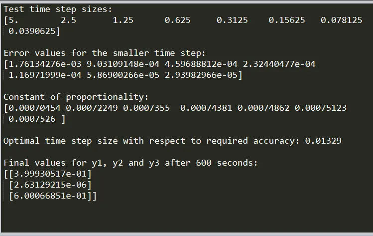
Fig(a) Console result display.
It can be observed that the initial time step size taken was 5. The smaller time step was half of the larger time step. In order to compute the ideal time step size, the fundamental behaviour of the time step with respect to error must be observed. For clarity, the formulae shown in Step VI will be shown again below.
`text(e) = ((y_(dt_1) -y_(dt_2)))/(2^k - 1)`
where,
`dt_1= text(time step size 1)`
`dt_2= text(time step size 2)`
`text(e = error value = error of the smaller time step)`
`dt_2 = dt_1/2`
The value of 'y' is obtained by using the function that solves the Newton-Raphson multivariate method, for two time steps considered. The maximum absolute value among the difference between `y_1,y_2` and `y_3` of the two time steps is taken, in order to obtain the error. The error value that is obtained after solving the equation, is the error present in the smaller time step size. Keeping this in mind, the results obtained will be observed.
For every time step considered, the error values of the current time step size seems to be around half of the error value of the previous time step size. The interesting part about this behaviour is that the time step size progression itself, is always half of the previous value. This suggests that the time step size and the error associated with it, are directly proportional. This has been shown below.
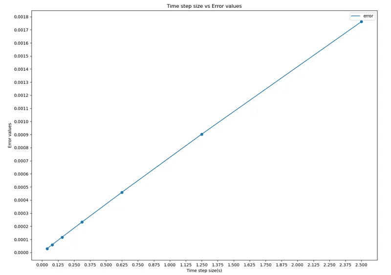
Fig(b) Plot for time step size vs error values.
In the figure above, it can be observed that the error values vary almost linearly with the time step size. This re-enforces the point stated above.
Mathematically,
`text(e) prop dt`
In order to equate these two terms, some constant of proportionality should be introduced.
`text(e ) = c*dt`
In this case, the equation becomes,
`text(e) = c*(dt_2)`
`c = text(e)/(dt_2)`
If the list for the constant of proportionality calculated for each time step size is observed, it can be seen that the values obtained are nearly the same.
After obtaining this constant of proportionality, the accuracy required must be determined. Higher accuracy requires a smaller time step, and will increase computational time. Since the constant of proportionality and the required accuracy are known to us, the optimal time step can be obtained from the same formula shown above, by simple rearrangement. Only instead of determining the error, the error introduced to the simulation is user defined. This has been shown below.
`dt_(ideal)= text(accuracy required)/c`
For this case, the accuracy is set to `10^5`.
Upon solving this equation, the ideal time step size is obtained, and has been displayed below.
Ideal time step size = 0.01329 s
Using this time step size, the ODEs are solved using the Implicit Euler method.
(b) Plot for time vs numerical solution of the ODEs (`y_1,y_2` and `y_3`)`
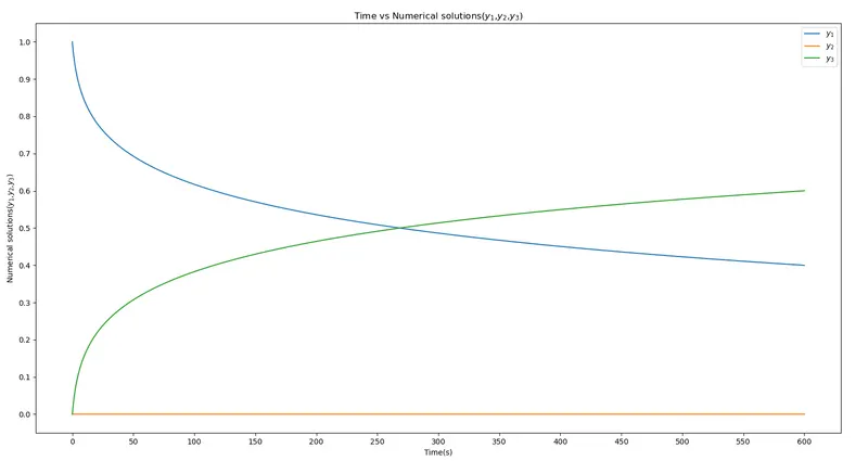
Fig(c) Plot for time vs numerical solution of the ODEs (`y_1,y_2` and `y_3`)`
This plot displays the behaviour of the numerical solutions of `y_1,y_2` and `y_3`.
The behaviour of of the numerical solutions of `y_1 and y_3` are interesting, as both of the plots seem like mirror images of each other, despite having very different equations. This behaviour can be attributed to the fact that they are coupled ordinary differential equations, and their behaviour is not entirely independent of each other.
If the behaviour of `y_1` and `y_3` are observed, it is understandable why the plot of `y_2` behaves in this fashion, as the ODE of `y_2` contains ODEs of both,`y_1` and `y_3`,albeit with a difference in their signs.